Menu
Downslope windstorms and high-drag states
Downslope windstorms in flow over mountains are associated with high-drag states. Using the drag exerted on the flow as a proxy for windstorm intensity is attractive since it is a single quantity for the whole flow field, which broadly reflects the magnitude of the wind speed enhancement on the lee side of the mountain.
High-drag states are better understood in idealized settings. One example is the following wind proile:
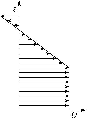
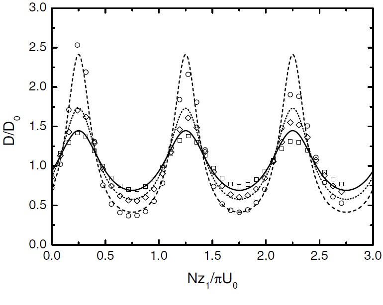
Figure 2 shows the drag normalized by its hydrostatic linear value for a constant wind equal to the surface wind U0, as a function of Nz1/(πU0), where N is the Brunt-Vaisala frequency of the incoming flow, for different values of the Richardson number Ri=N2/(dU/dz)2 in the upper layer. In linear conditions, drag maxima occur for Nz1/(πU0)=0.25+n (where n is an integer), and are more pronounced as Ri decreases.
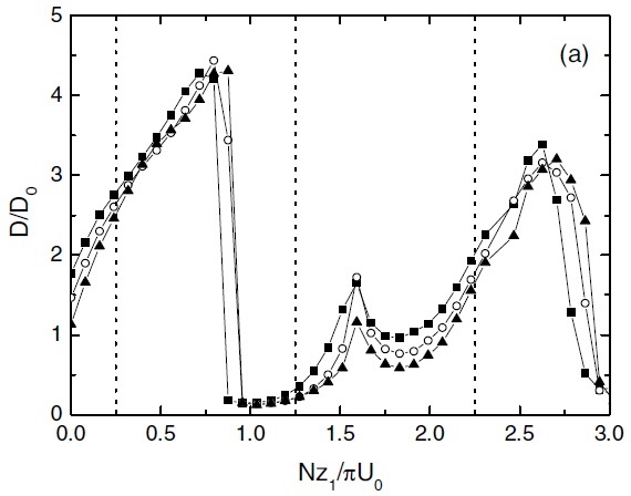
In weakly nonlinear conditions for which Nh0/U0=0.5 (where h0 is the mountain height) (Figure 3), the dependence on Ri weakens, the maxima are translated to higher values of Nz1/(πU0), and the maxima occuring in Figure 2 at Nz1/(πU0)=1.25+2n almost disappear. This is clearly due to nonlinear effects, and is a phenomenon still under debate, as pointed out by (Teixeira 2014)
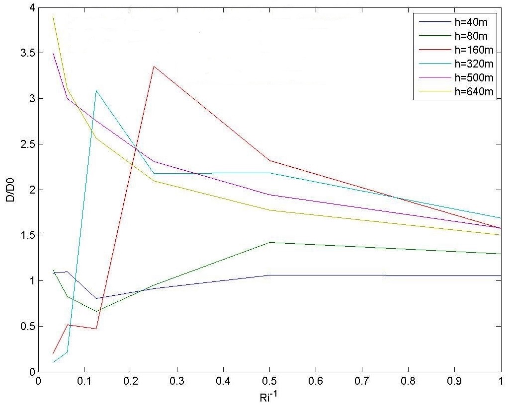
The wind profiles presented in Figures 4 and 5 vary linearly near the surface and are constant in an upper layer. The difference is that in Figure 5 there is a critical level (where the wind speed vanishes) below the height where the wind becomes constant (i.e., the shear is negative), while in Figure 4 no critical level exists, as the shear is positive.
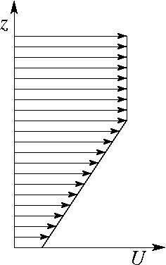
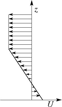
Figure 6 shows that the behaviour of the drag is quite different for these two wind profiles. While for positive shear the drag increases with Ri-1 for a given ratio of the velocity in the constant wind layer U1 and at the surface U0, for negative shear with a critical level the opposite happens. In weakly nonlinear flow (Nh0/U0=0.5), the drag is more enhanced in the first case at low Ri, but more enhanced in the second case at high Ri. This nonlinear phenomenon needs to be understood.
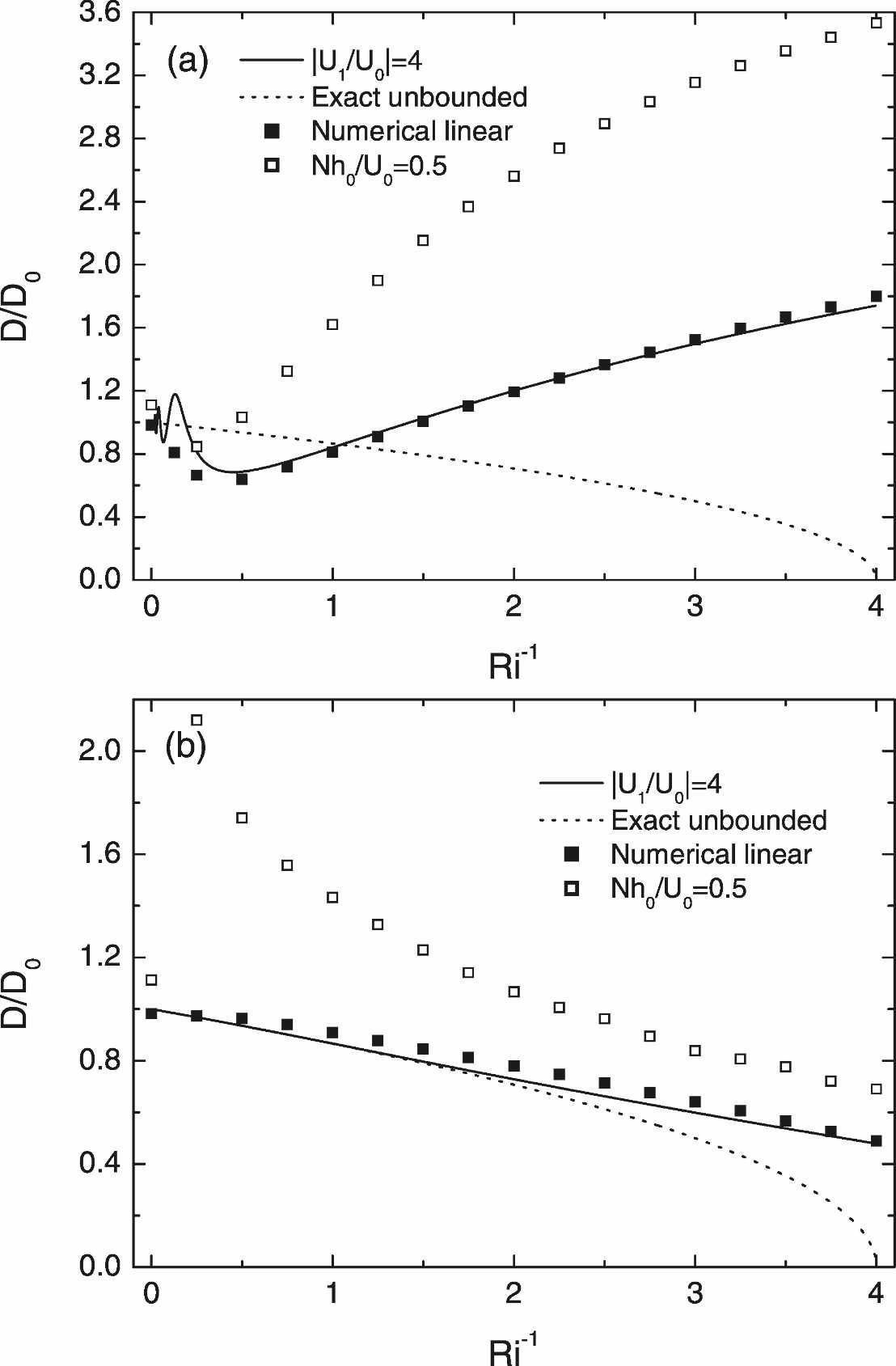
The case where the drag is amplified in flows with large Ri and a critical level (Figure 6(b)) is especially relevant, because it shows that weak shear can have a strong impact on the drag, and hints towards a long-distance interaction between the orography and the critical level.
Additional numerical simulations were carried out to explore further this effect. Figures 7 and 8 show these results. It can be seen that the drag oscillates for high values of Ri, and tends to be amplified substantially with respect to its linear estimate even for relatively low values of Nh0/U0.
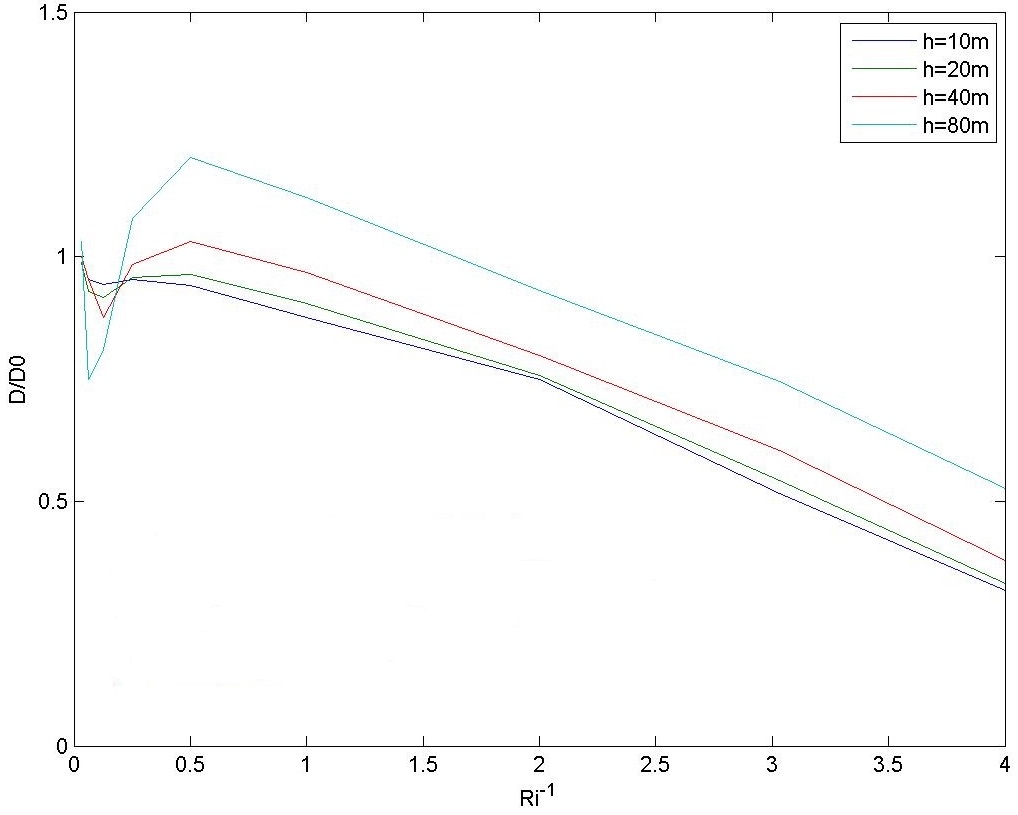
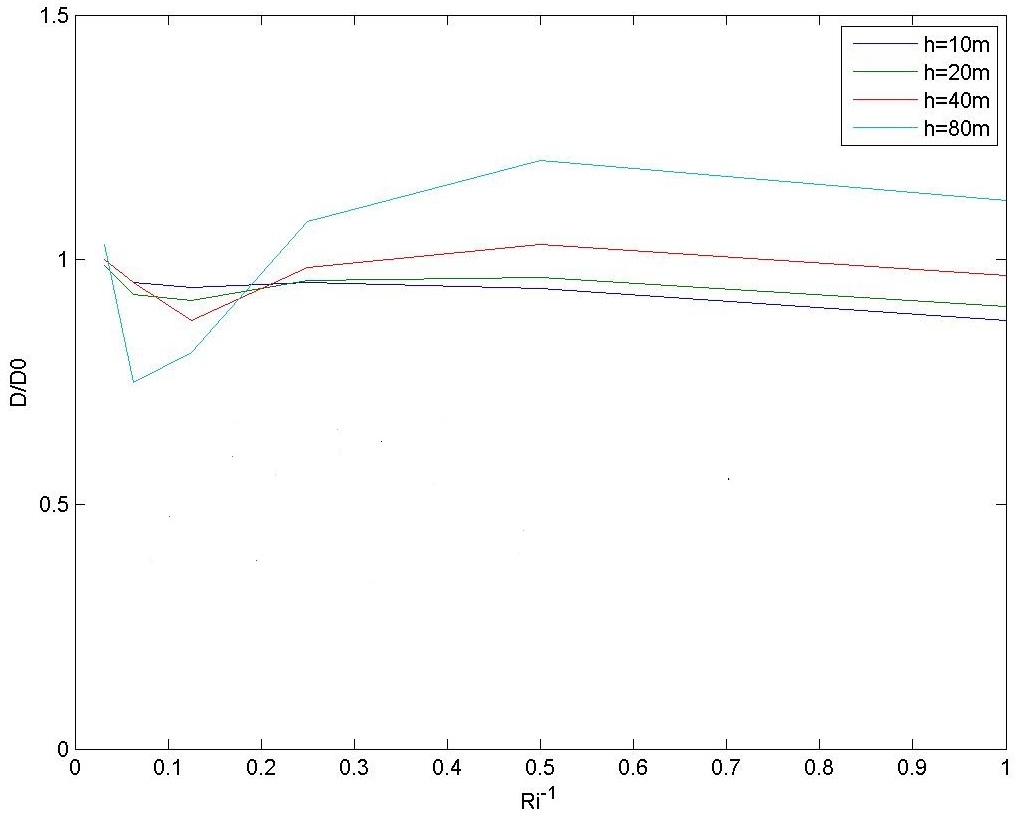
For higher values of Nh0/U0 (Figure 8), the drag amplification can be very large, and the values of Ri for which there existed attenuation of the drag instead of amplification for lower values of Nh0/U0 tend to disappear.
It is possible to calculate a wave reflection coefficient from the drag modulation shown in these graphs, and this will be included in a paper currently in preparation. This gives us indications about how critical levels may shift from being absorbing, for low amplitude mountain waves, to reflective, for higher amplitude waves, as shown anecdotally by Breeding (1971).
Downslope windstorms may be also be generated in two-layer fluids (where the interface between the two layers represents, for example, an atmospheric inversion). An example is given in the paper by Baines and Johnson (2016) included in the special issue of Frontiers in Earth Science on "The Atmosphere over Mountainous Regions" (Teixeira et al. 2016). Another example is provided by the recent study of Teixeira et al. (2017), which compared laboratory experiments of the drag with linear theory, for a flow with two layers of constant (distinct) density.
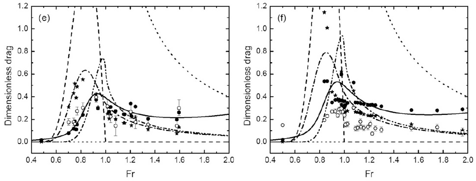
Figure 9 shows a comparison between results from various versions of linear theory (lines and filled symbols) and laboratory experiments (open circles). The drag attains a large maximum for Fr ≈ 1, which corresponds to a kind of resonance when the phase speed of the dominant waves matches the mean flow speed.
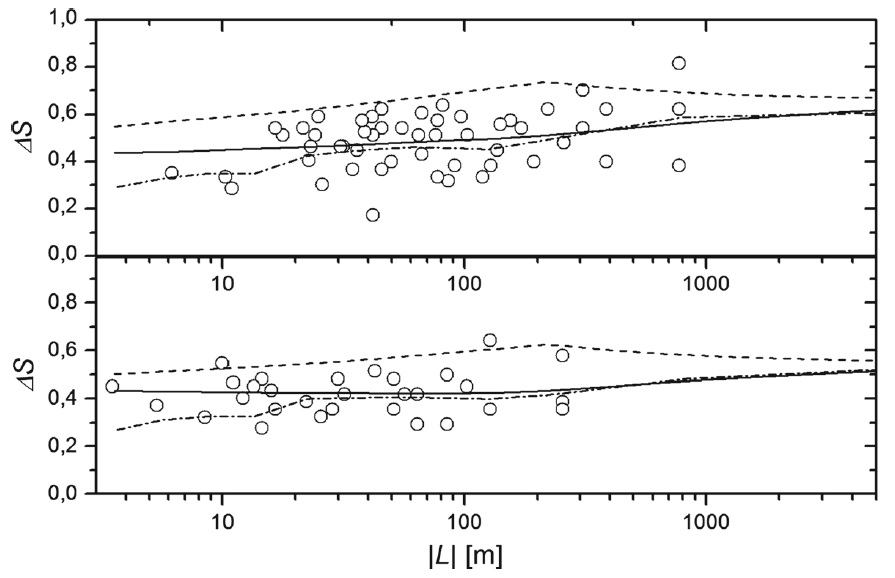
Downslope winds are strongly influenced by boundary layer effects. The boundary layer behaves differently under stable or unstable stratification. Following Argain et al. (2009), Argain et al. (2017) developed a model of how the flow speed-up (the ratio of the velocity disturbance to the mean velocity at a given level) varies as a function of the Obukhov length L (a measure of the static stability). This is illustrated for a statically unstable flow in Figure 10.