Menu
Trapped lee waves and rotors
Conditions for the generation of rotors beneath trapped lee waves are not well understood. Vosper (2004) and Sheridan and Vosper (2006) presented regime diagrams indicating for what combination of parameters different flow structures (including rotors) could be detected in their numerical simulations downstream of an isolated mountain for the atmospheric profile shown in Figure 1.
Teixeira et al. (2013) showed that the drag associated with trapped lee waves propagating at the inversion correlated fairly well with regions in parameter space where rotors occur. This is shown in Figure 2. Note that the drag, despite being very small, has maxima that roughly coincide with the occurrence of rotors.
In order to get a more physically-based estimate for the onset of rotors, the natural choice is to compute the conditions for flow stagnation downstream of the mountain. However, the impact of the velocity boundary-layer on this calculation is crucial. Teixeira (2017) developed a model including this effect by combining the inviscid trapped lee wave model of Teixeira et al. (2013) with the bulk boundary layer model of Smith et al. (2006).
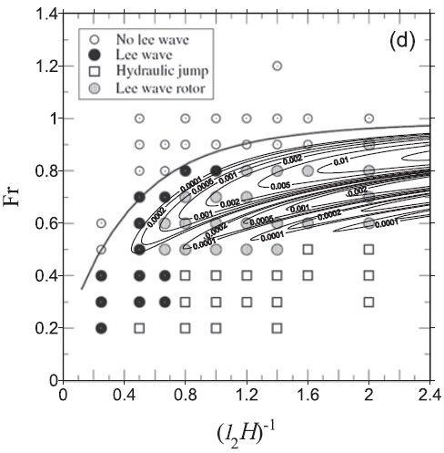
Figure 3. shows the inverse of the critical dimensionless mountain height (l2h0)crit for flow stagnation from linear theory, superposed on the regime diagram of Vosper (2004). Since that author used l2h0=0.5 in their simulations, the contour 2 of (l2h0)crit-1 should enclose the zone of parameter space where rotors occur. The value of this quantity is clearly underestimated in Figure 3(a), where a totally inviscid version of the model is used and 3(b) for an improved model, where the velocity perturbation amplification and mean flow attenuation in the boundary layer are taken into account, but produces fairly good agreement only in Figure 3(c), where the complete model with feedback of the boundary layer on the inviscid atmosphere is used. However, flow stagnation is also predicted in zones where a hydraulic jump occurs.
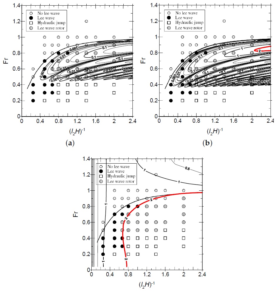
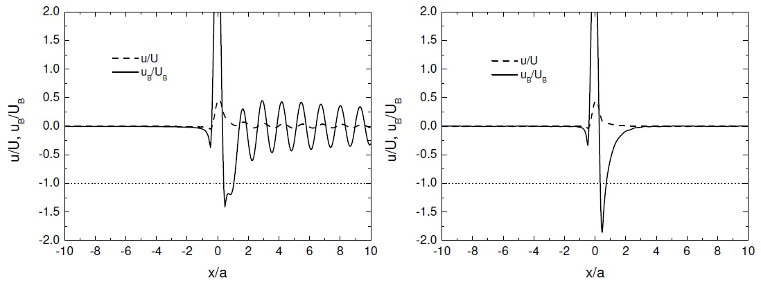
Figure 4 shows the velocity perturbation (normalized by the mean velocity) inside the boundary layer (solid lines) and outside it (dashed lines) (denoted by uB/UB and u/U, respectively) for the 3 cases illustrated in Figures 4, 5 and 8 of Vosper (2004). While inside the boundary layer flow stagnation is predicted in Figure 4(b), as happens in the numerical simulations, the reasons for this stagnation do not seem physically correct, as there are no trapped lee wave signatures in the velocity perturbations. Flow stagnation never occurs outside the boundary layer, which illustrates the crucial importance of friction.
A different, less hydrostatic case (with a narrower mountain), numerically simulated by Sheridan and Vosper (2006), is illustrated in Figure 5. It can be seen that the inviscid version of the model (Figure 5(a)), but especially its improved version (Figure 5(b)) predict much better the critical mountain height for rotor onset, although the full model produces a comparably good prediction. However, a the flow stagnation condition in the full model also diagnoses cases with a hydraulic jump in addition to rotors. It would be useful to develop a procedure to discriminate between these two different flow structures.
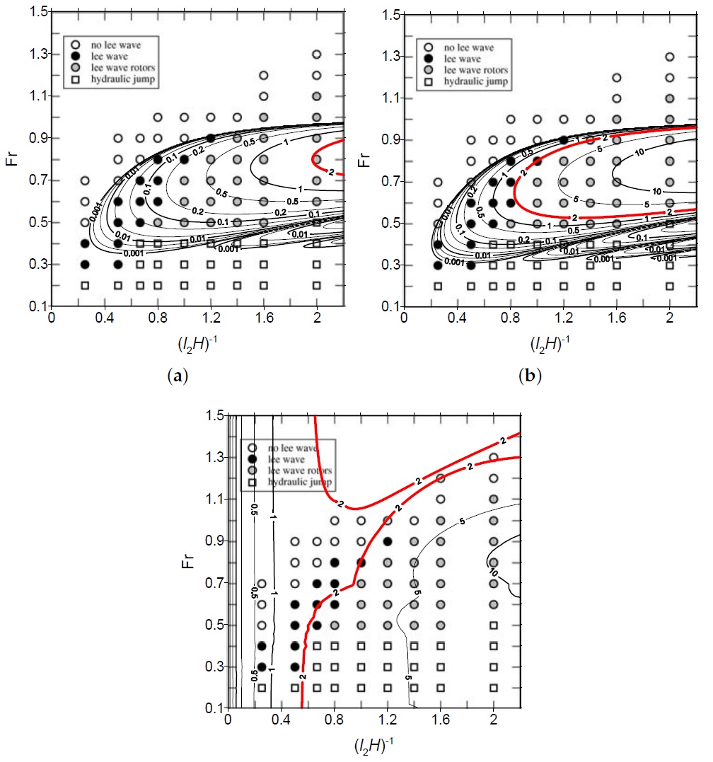
Figure 6 shows the normalized velocity perturbations corresponding to this flow, for a case where rotors and a hydraulic jump are predicted numerically ((a) and (b), respectively). The linear model now produces trapped lee waves in the first case, which is a sign that it captures better the physics of the flow, although there is still only one stagnation point.
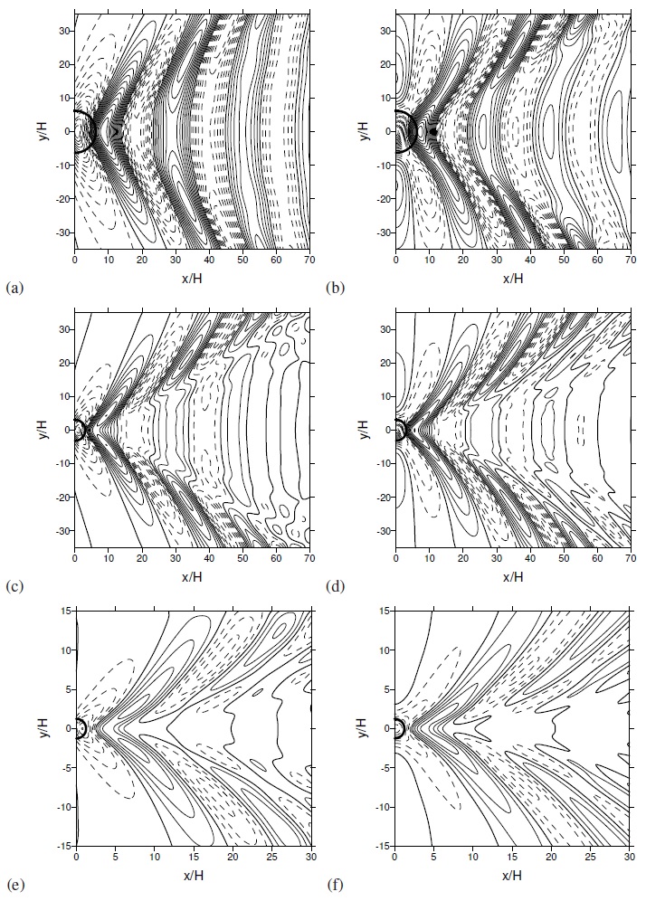
The drag produced by trapped lee waves has also been studied in Teixeira and Miranda (2017) (in press). This study extended previous 2D calculations to a 3D axisymmetric mountain. Figure 8 shows a comparison between the drag for the atmosphere of Scorer (1949), shown in Figure 7, obtained from linear theory and from numerical simulations. As l1a decreases (where a is the mountain width), i.e. the flow becomes more non-hydrostatic, the drag component associated with trapped lee waves increases relative to the drag associated with waves propagating upward in the upper layer (internal wave drag).
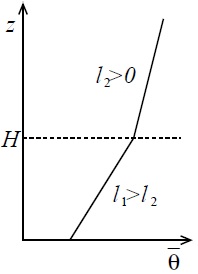
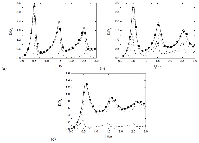
Figure 9 shows the normalized vertical velocity perturbation associated with the waves. The waves generated by an axisymmetric mountain look like ship waves, emanating from the orography, and spreading along a triangular wake, which is wider for more hydrostatic flow.
Apart from variations of stability, trapped lee waves can also be generated by winds that increase constinuously with height, forcing the waves to become progressively evanescent. Yu and Teixeira (2015) treated this situation. Figure 10 shows the normalized drag as a function of Ri for U1/U0=4 (where U0 and U1 are defined as in the section on downslope windstorms) and different values of Na/U0.
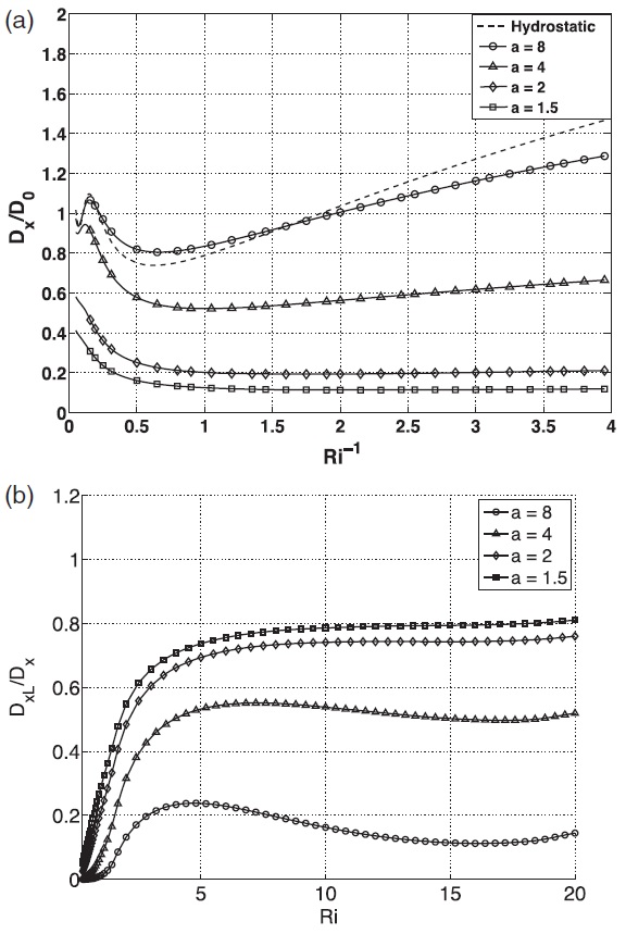
It can be seen that the trapped lee wave drag component is especially important at relatively low values of Na/U0 and high values of Ri, i.e., substantially non-hydrostatic flow and a relatively thick lower shear layer.