Menu
Mountain wave breaking and CAT generation
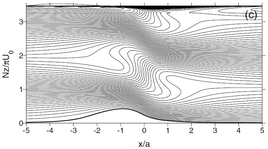
For an atmosphere with constant parameters, the conditions for flow stagnation or wave breaking over a 2D mountain are well known. They have also been studied using linear theory for 3D mountains by Smith (1989). Teixeira et al. (2005) noted that, for the wind profile of Figure 1 in the section "Downslope windstorms", the conditions for wave breaking change (see Figure 1), with flow overturning occuring in zones displaced laterally with respect to the mountain, at different altitudes, and for lower dimensionless mountain heights. This is due to constructive interference between the upward and downward propagating waves in the lower layer, reflected at the shear discontinuity.
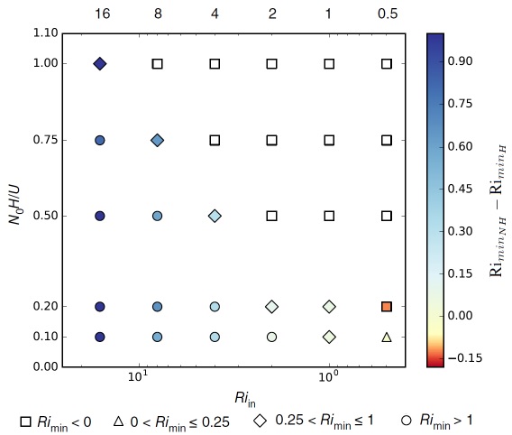
Guarino et al. (2016) studied the considerably more complicated problem of mountain wave breaking in flows with directional shear over axisymmetric mountains using numerical simulations. They developed a regime diagram (shown in Figure 2) where the Richardson number Ri of the flow affected by mountain waves is represented as a function of the Ri of the incoming background flow and the dimensionless mountain height, for wind profile 3 in Figure 1 of the section "Shear effects in mountain wave drag".
The regime diagram shows that the flow becomes more unstable as either Nh0/U0 increases, or the background Ri decreases, with most of parameter space occupied by either absolute stability (Ri>1) or static instability due to flow overturning (Ri<0).
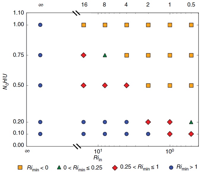
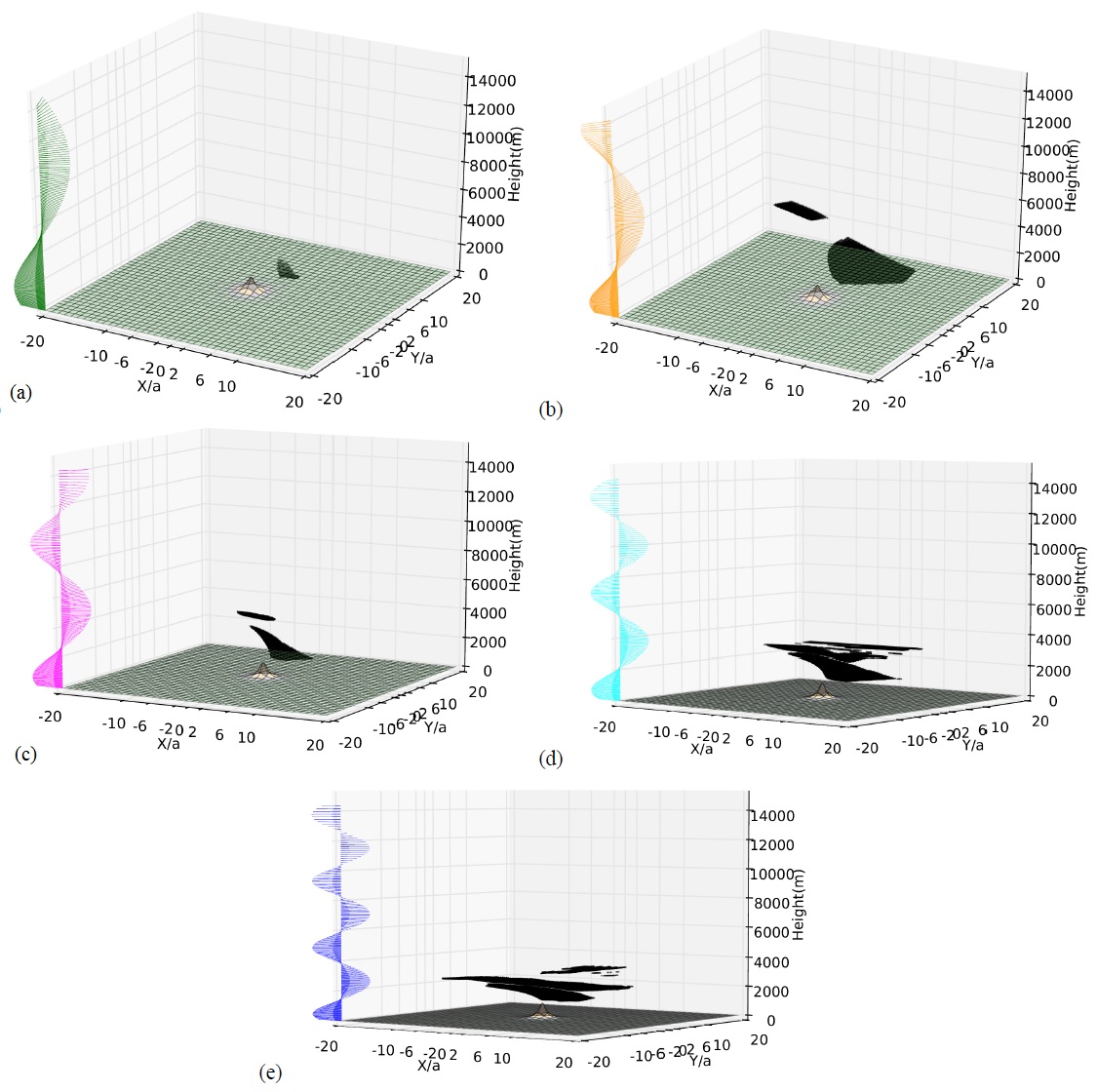
Figure 3 shows the distribution of regions near the orography where Ri<0.25, for Nh0/U0=1 and different values of the Richardson number of the background flow. It can be seen that, as the backgound Ri decreases, the regions of dynamical flow instability expand laterally, and they also tend to occur lower down in the atmosphere. This is because such regions are associated with the critical levels of the various waves present in the wave spectrum, and once the wind has turned by an angle of 180 degrees (which happens at lower levels for low background Ri), essentially no wave energy remains, as all waves have been dissipated.
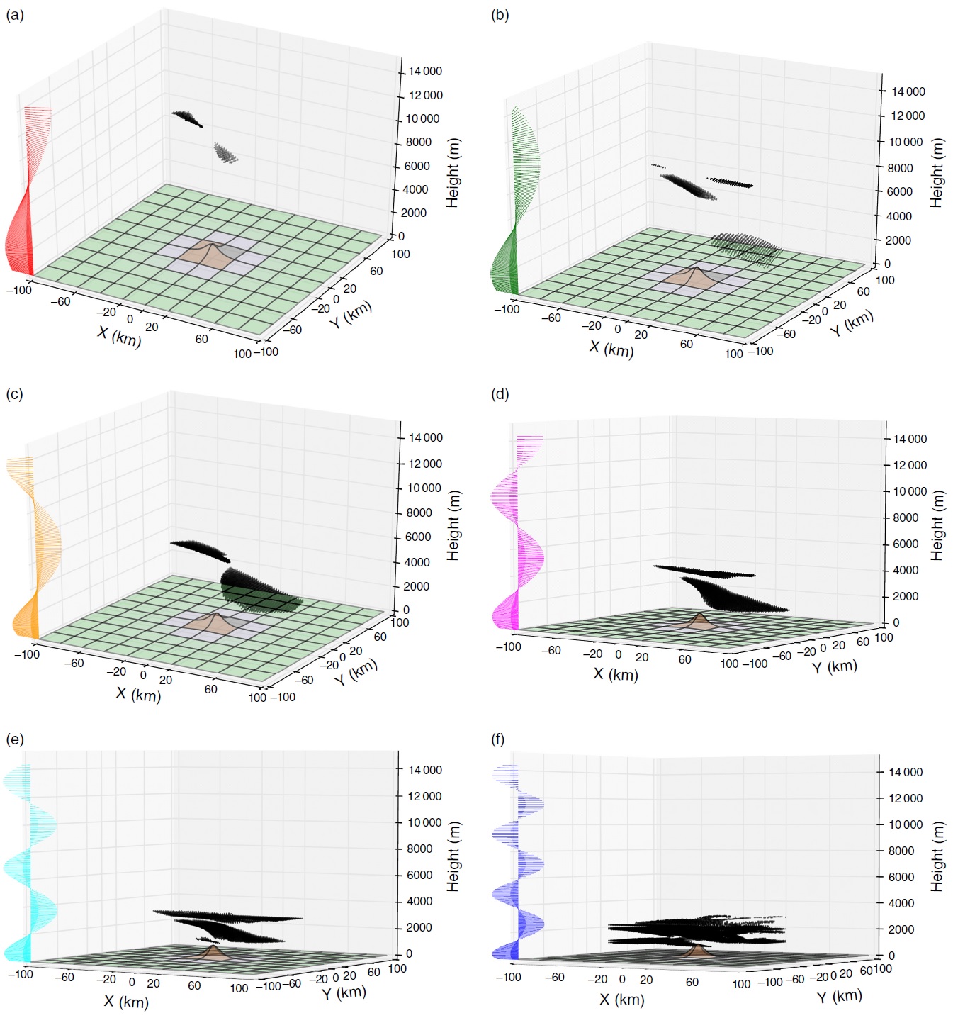
Figure 4 shows cross sections of the horizontal velocity field associated with the waves, at a height where wave breaking is occuring. The velocity perturbation vector is perpendicular to the background wind vector in the most unstable region (left panel). This is confirmed by the right panel, where the angle between the mean and perturbation velocity vectors indeed takes values near 90 degrees in the region where Ri<0.25. This might form the basis for a new mountain wave turbulence diagnostic.
Guarino and Teixeira (2017) evaluated the impact of non-hydrostatic effects on wave breaking in directional shear flows, using the same wind profile and orography shape, but a narrower mountain. Figure 5 shows a regime diagram similar to that of Figure 2, but where differences of stability between the hydrostatic and non-hydrostatic flow are also indicated by the colours.
The flow becomes more stable for a narrower mountain for high values of the background Ri, but for the lowest values (namely Ri=0.5) it becomes more unstable (i.e. the minimum Ri of the total flow decreases). This happens because, while for high background Ri the waves have to travel a large vertical distance before they break, and in the meantime are weakened by dispersion, for the lowest background Ri, the waves break at low levels, so dispersion does not have the time to act. Additionally, the waves have higher amplitude near the ground than in the hydrostatic case, because of the steeper slope of the orography.
This is confirmed by Figure 6, where the regions near the mountain where Ri<0.25 are shown for this more non-hydrostatic flow. The regions of dynamic instability (Ri<0.25) are clearly closer to the surface for high background Ri, consistent with the effect of dispersion in weakening the waves as they propagate upward. Unstable regions also seem to be more concentrated near the mountain for low Ri.
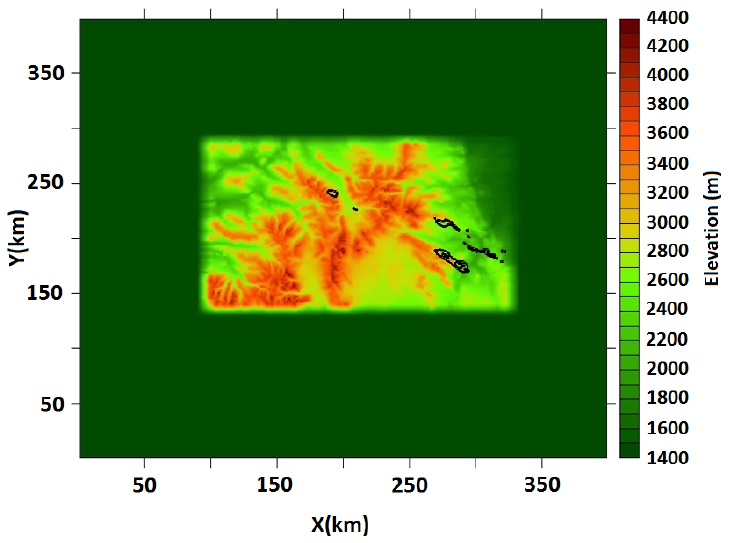
Guarino et al. (2017) (submitted paper, under revision) also addressed a more specific case study of turbulence thought to be generated by mountain wave breaking over the Rocky mountains, using semi-idealized numerical simulations. Figure 7 shows the regions over the mountains where there is static instability (Ri<0) (and hence turbulence should be generated) from simulations that used only the displayed portion of the Rocky Mountains as lower boundary condition, and an upstream sounding to define the wind and stability in the background flow. The elongated wake of instability suggests directional shear as the mechanism responsible for wave breaking.
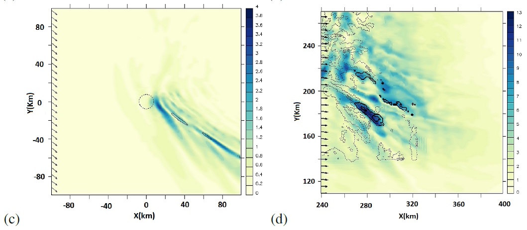
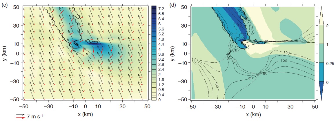
This idea is made plausible by Figure 8, where cross sections of the horizontal velocity perturbation and zones of static instability are shown at levels where wave breaking is predicted, for an idealized flow with directional shear (left panel) and for the more realistic simulations of flow over the Rocky Mountains. Clearly the asymptotic wake (Shutts 1998) visible on the left panel has a counterpart in the more realistic flow represented on the right panel.
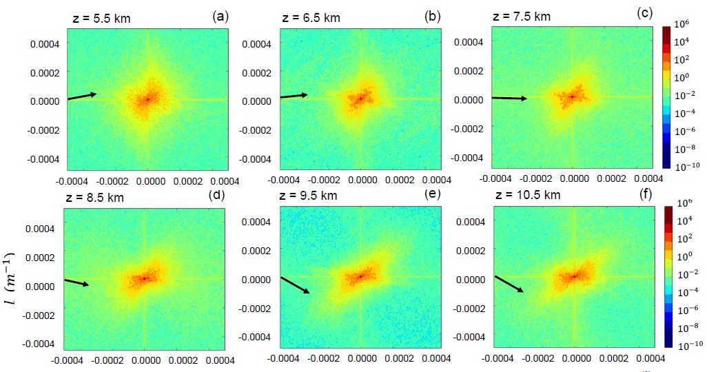
Figure 9 shows spectra of the horizontal velocity perturbation that further corroborate this point. It can be seen that the energy in these spectra rotates clockwise in wavenumber space, accompaying the background wind rotation, and concurrently decreases in magnitude, which corresponds to an energy loss by wave breaking. This is especially visible between z=5.5km and z=7.5km (the altitude of diagnosed wave breaking). All of this is consistent with the dynamics of critical levels, as understood from linear theory.