Advanced Use

Here are some hints and tips on advanced use of cf-plot.

Adding user defined lines and text to plots

In cf-plot the plot is stored in a plot object with the name cfp.plotvars.plot. The page containing the plots is named cfp.plotvars.plot_master.

To see all the methods for the plot object type

cfp.gopen()
dir(cfp.plotvars.plot)

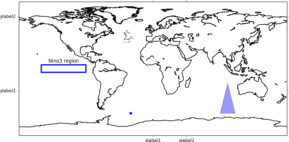
In this example we make a blank map plot, change the longitude labels and add a box and some text. To add text and lines outside of the plot use the same method as below with coordinates outside of the defined plot area.

import cf
import cfplot as cfp
import matplotlib
from matplotlib.patches import Polygon
from matplotlib.collections import PatchCollection

f=cf.read('/opt/graphics/cfplot_data/tas_A1.nc')[0]

cfp.gopen()
cfp.levs(-1000, -900, 100)
xticks=[0.0, 45.0]
xticklabels=['xlabel1', 'xlabel2']
yticks=[-30.0, 70.0]
yticklabels=['ylabel1', 'ylabel2']

cfp.con(f.subspace(time=15), fill=False, colorbar=None,
    xticks=xticks, xticklabels=xticklabels,
    yticks=yticks, yticklabels=yticklabels)

# A box
xpts=[-150, -150, -90, -90, -150]
ypts=[-5, 5, 5, -5, -5]
cfp.plotvars.plot.plot(xpts,ypts, linewidth=3.0, color='blue')

# A symbol
cfp.plotvars.plot.plot(-30,-60, linewidth=3.0, marker='o', color='blue')

# Text
cfp.plotvars.plot.text(-120, 8, 'Nino3 region', horizontalalignment='center')

# Equation
cfp.plotvars.plot.text(-40, 40, r'$\sum_{i=0}^\infty x_i$')

# Filled polygon
box=[[90, -60], [100,-20], [110, -60]]
patches = []
polygon = Polygon(box, True)
patches.append(polygon)
p = PatchCollection(patches, cmap=matplotlib.cm.jet, alpha=0.4)
cfp.plotvars.plot.add_collection(p)

cfp.gclose()

Manually changing colours in a colour scale

The simplest way to do this without writing any code is to modify the internal colour scale before plotting. The colours most people work with are stored as red green blue intensities on a scale of 0 to 255, with 0 being no intesity and 255 full intensity.

White will be represented as 255 255 255 and black as 0 0 0.

The internal colour scale is stored in cfp.plotvars.cs as hexadecimal code. To convert from decimal to hexadecimal use hex i.e. hex(255)[2:] ‘ff’

The [2:] is to get rid of the preceding 0x in the hex output.

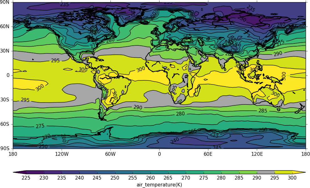
For example, to make one of the colours in the viridis colour scale grey use:

import cf
import cfplot as cfp
f=cf.read('/opt/graphics/cfplot_data/tas_A1.nc')[0]
cfp.cscale('viridis', ncols=17)
cfp.plotvars.cs[14]='#a6a6a6'
cfp.con(f.subspace(time=15))

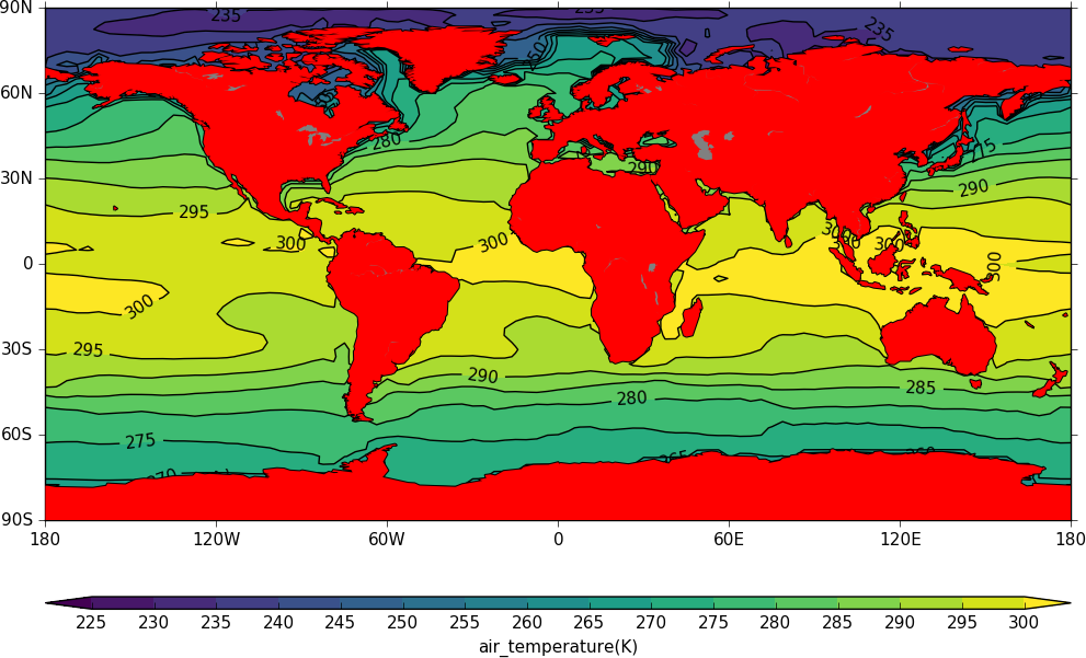
Colouring land and lakes

This is done by changing the land_color and lake_color variables in cfp.setvars.

import cf
import cfplot as cfp
f=cf.read('/opt/graphics/cfplot_data/tas_A1.nc')[0]
cfp.setvars(land_color='red', lake_color='grey')
cfp.con(f.subspace(time=15))

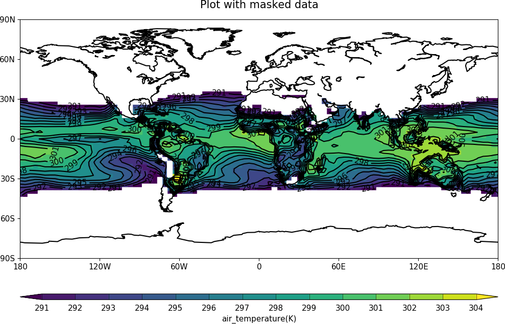
Plotting missing data

Masked data isn’t plotted.

import cf
import cfplot as cfp
import numpy as np


f = cf.read('/opt/graphics/cfplot_data/tas_A1.nc')[0]
g = f.subspace(time=15)


# Mask off data less that 290 K
h = g.where(g<290, cf.masked)


# Normal plot with masked data
cfp.con(h, blockfill=True, title='Plot with masked data')

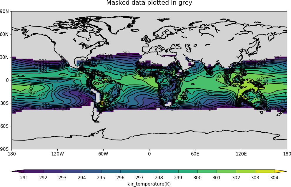
Masked data is plotted as blockfill in grey.

# Turn off the hardmask and set masked points to 999
h.hardmask=False
i = h.where(h.mask, 999)


# Open a plot with gopen as we will be plotting over a contour plot
cfp.gopen()
cfp.con(h, blockfill=True, title='Masked data plotted in grey')


# Call internal block filling routine
cfp.bfill(f=np.squeeze(i.array), x=i.item('X').array, y=i.item('Y').array,
          clevs=[990, 1000], lonlat=True, single_fill_color='#d3d3d3')


cfp.gclose()

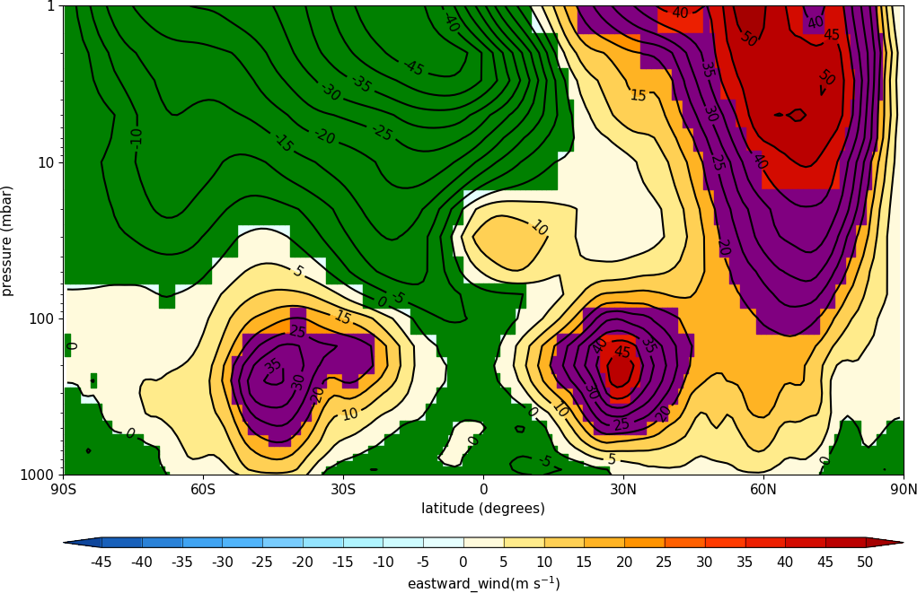
Blockfill with individual colours

If a plot needs to be built up as a series of blockfill plots then this is possible using the cf-plot internal blockfill routine.

f=cf.read('/opt/graphics/cfplot_data/ggap.nc')[1]
g=f.collapse('mean','longitude')




x=g.item('Y').array
y=g.item('Z').array
data=np.squeeze(g.array)


cfp.gopen()
cfp.con(g, ylog=True)

# Call internal block filling routine
cfp.bfill(f=data, x=x, y=y, clevs=[-50, 0], single_fill_color='green')

cfp.bfill(f=data, x=x, y=y, clevs=[20, 40], single_fill_color='purple')
cfp.gclose()