WS Test program results
Ross Bannister, September 2004, October 2004- This page is found at "www.met.rdg.ac.uk/~ross/DARC/WS/OffLineText1.html" on the www (Reading access only)
- and at "file:///home/mm0200/frxb/public_html/WS/OffLineText1.html" on the Met Office intranet.
Page last updated 18th October 2004. This page now includes results for streamfunction, temperature and zonal wind. The experiment IDs have changed from the previous version.
1. Introduction
In Var., background error covariances are represented as a set of control variable transforms. Any approach to modelling the transforms in this way leads to approximations which come to light in analyses of the implied covariances. A good background error covariance model should reproduce the position and scale dependencies of forecast errors. The background error covariance model used currently in Var. is unable to achieve this task well, but it is supposed that the scope of a background error model to capture both position and scale dependencies simultaneously is improved by using a waveband (or wavelet-like) approach, called the "waveband summation" (WS) method.In [VWP19], a number of WS models are discussed, and are summarized at the start of section 6 in [Bannister]. In the rest of [Bannister], the formulation of one particular waveband model - the simplest - is studied in detail. This includes the transform definition, its pseudo-inverse (it has no exact inverse) and possible procedures for determining the many coefficients in the transforms, which can be estimated by running pairs of forecasts (or NMC runs).
In preparation for a publication of this work, this document presents results from a simple cut-down and off-line version of the WS transform run at Reading. Investigations have been performed into the ability of the WS transform to capture the position and scale dependencies of forecast errors and the accuracy of the pseudo-inverse transform. The results are compared to other representations of background errors - the 'exact' approach (ie the explicit B-matrix for the cut-down system) and the current Met Office spatial transforms (see sections 4.2 and 4.3 of [Bannister]).
The structure of this document is as follows. In section 2 we review the version of the WS transform used, and in section 3 we describe the experiments used to diagnose the properties of this model. Section 4 presents the results and section 5 describes them. Section 6 makes some final comments.
References
- [VWP19] Andrews P.L.F., Lorenc A.C., On introducing a multi-scale waveband-summation covariance model into the Met Office Var system, Var. Working Paper 19 (2002).
- [Bannister] Bannister R.N., On control variable transforms in the Met Office 3d and 4d Var., and a description of the proposed waveband summation transformation, gzipped postscript or pdf (2004).
- [Ingleby] Ingleby N.B., The statistical structure of forecast errors and its representation in the Met Office global 3d-Var scheme, QJRMS 127, pp. 209-231 (2001).
2. The WS transform, the data and the methodology
In the following lists, equation, figure and section numbers refer to [Bannister], unless indicated otherwise.The transform used
- The WS U-transform used is shown as Eq. (72) and is described in section 6, but is used here with no parameter transform.
- Some multi-band transforms proposed in [VWP19] use multiple control vectors, the one used here has only one.
- In the vertical transform used in WS, the modes have been rotated back to model levels (section 4.2.2).
- One vertical transform is used per latitude point in the forecast difference fields, as opposed to using one vertical transform per latitude band.
- Identity inner products have been used throughout for simplicity.
- We use an undersized last bandpass function (section 6.2.2).
- No spectral correction function (ie 'gamma' in [VWP19]) has been used in the calibration.
- We have the option to use triangular or top-hat band-pass functions and can control separately those used in the U and approximate T-transforms.
- ECMWF ERA-40 forecast differences have been used to calibrate the transforms (ie to determine the vertical EOFs, their variances and the horizontal spectra). We use these because we have them to hand.
- ECMWF fields are at a high resolution (480 x 240 x 60). For our problem to be practical, these are reduced to (80 x 40 x 30).
- The ECMWF convention of labelling the vertical levels from the top of the model is reversed here to match the MetO convention.
- We are not doing assimilation - but we are looking at diagnostics that show some of the covariances implied by the WS transform.
- We also evaluate how invertible the WS transform is.
- The problem is demanding on memory and so a three-dimensional problem of reasonable resolution cannot be dealt with on a workstation.
- A two-dimensional version is implemented - latitude vs. height. This still allows study of the variation of errors with horizontal and vertical position and scale.
- For the purposes of calibrating the statistics, averages are made over longitude instead of averages over realizations. Each longitude slice of a 3d field is considered to be a realization.
- The statistics are calibrated for one forecast difference field (actually in January). We are comparing different methods of representing forecast errors and this is expected to be adequate for a first test.
- There is no parameter transform - this study looks only at spatial and scale dependencies of errors.
- Simple fourier transforms in latitude are used to convert between horizontal position and horizontal scale.
- For comparison, the same methodology is used to diagnose all of the transforms considered (the full explicit B-matrix representation, the current Met Office version and the WS transform).
3. The experiments
What representations of B are used?
- A full, exact representation of B (called 'Exact'). This is actually the explicit B matrix.
- The Met Office's current transforms (called 'MetO').
- The WS transform described above (called 'WS').
- Implied variances of streamfunction, temperature an zonal wind as a function of latitude and model level (like Fig. 4 of [Ingleby]).
- Implied vertical correlations of streamfunction, temperature and zonal wind with a given model level (around 500 hPa) as a function of horizontal wavenumber and model level (like Fig. 2 of [Ingleby]).
- The number of bands can be changed.
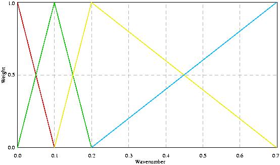
- We consider the 'optimal' case (where the typical lengthscale of each band is equal to the band width). For our system, the optimal case has four bands (see Fig. below).
- We also consider extreme cases of one band and ten bands.
- The shape of the bands can be either triangular (Fig. 10) or top-hat (Fig. 11). We try out:
- triangular band shapes in the T and U-transforms,
- top-hat band shapes in the T and U-transforms, and
- top-hat band shapes in the T-transform and and triangular band shapes in the U-transform.
- Note: the T-transform is used during calibration and the U-transform is used for the implied variances/covariances diagnostics. Both are used for the inverse transform tests.
The WS transform has no exact inverse. What tests have been done to assess the validity of the approximate inverse (section 6.3)?
- We operate systematically with UT and UT on a delta function to see if the delta-function is recovered.
- We plot the resulting field of UT acting on a delta function at a particular latitude/height, and the resulting field of TU acting on a delta function at a particular wavenumber/height.
- We plot effective submatrices of UT and TU (the complete matrix is too complicated to plot).
- Note: the approximate inverse, T, has been designed to work as TU, not as UT.
- During calibration, some of the vertical covariance matrices have very small eigenvalues. Numerical error has caused some of these to become negative. This creates a problem when they are square-rooted. The associated modes are ignored in the transforms, but they will contribute to the transforms being non-invertible. More later.
| ID | B-model | Quantity | No. bands | T bandshape | U bandshape | My Ref. |
| -- | ------- | -------- | --------- | ----------- | ----------- | ---- |
| Ap | Exact | psi | n/a | n/a | n/a | Runs_for_doc1/Run1/ |
| At | Exact | T | n/a | n/a | n/a | Runs_for_doc1/Run1T/ |
| Au | Exact | u | n/a | n/a | n/a | Runs_for_doc1/Run1u/ |
| -- | ------- | -------- | --------- | ----------- | ----------- | ---- |
| Bp | MetO | Streamfn | n/a | n/a | n/a | Runs_for_doc1/Run2/ |
| Bt | MetO | T | n/a | n/a | n/a | Runs_for_doc1/Run2T/ |
| Bu | MetO | u | n/a | n/a | n/a | Runs_for_doc1/Run2u/ |
| -- | ------- | -------- | --------- | ----------- | ----------- | ---- |
| Cp(*) | WS | psi | 4 | Top-hat | Triangular | Runs_for_doc1/Run3/ |
| Ct(*) | WS | T | 4 | Top-hat | Triangular | Runs_for_doc1/Run3T/ |
| Cu(*) | WS | u | 4 | Top-hat | Triangular | Runs_for_doc1/Run3u/ |
| -- | ------- | -------- | --------- | ----------- | ----------- | ---- |
| Dp | WS | psi | 4 | Top-hat | Top-hat | Runs_for_doc1/Run6/ |
| Dt | WS | T | 4 | Top-hat | Top-hat | Runs_for_doc1/Run6T/ |
| Du | WS | u | 4 | Top-hat | Top-hat | Runs_for_doc1/Run6u/ |
| -- | ------- | -------- | --------- | ----------- | ----------- | ---- |
| Ep | WS | psi | 4 | Triangular | Triangular | Runs_for_doc1/Run7/ |
| Et | WS | T | 4 | Triangular | Triangular | Runs_for_doc1/Run7T/ |
| Eu | WS | u | 4 | Triangular | Triangular | Runs_for_doc1/Run7u/ |
| -- | ------- | -------- | --------- | ----------- | ----------- | ---- |
| Fp | WS | psi | 1 | Top-hat | Triangular | Runs_for_doc1/Run8/ |
| Ft | WS | T | 1 | Top-hat | Triangular | Runs_for_doc1/Run8T/ |
| Fu | WS | u | 1 | Top-hat | Triangular | Runs_for_doc1/Run8u/ |
| -- | ------- | -------- | --------- | ----------- | ----------- | ---- |
| Gp | WS | psi | 2 | Top-hat | Triangular | Runs_for_doc1/Run10/ |
| Gt | WS | T | 2 | Top-hat | Triangular | Runs_for_doc1/Run10T/ |
| Gu | WS | u | 2 | Top-hat | Triangular | Runs_for_doc1/Run10u/ |
| -- | ------- | -------- | --------- | ----------- | ----------- | ---- |
| Hp | WS | psi | 3 | Top-hat | Triangular | Runs_for_doc1/Run4/ |
| Ht | WS | T | 3 | Top-hat | Triangular | Runs_for_doc1/Run4T/ |
| Hu | WS | u | 3 | Top-hat | Triangular | Runs_for_doc1/Run4u/ |
| -- | ------- | -------- | --------- | ----------- | ----------- | ---- |
| Ip | WS | psi | 10 | Top-hat | Triangular | Runs_for_doc1/Run9/ |
| It | WS | T | 10 | Top-hat | Triangular | Runs_for_doc1/Run9T/ |
| Iu | WS | u | 10 | Top-hat | Triangular | Runs_for_doc1/Run9u/ |
| -- | ------- | -------- | --------- | ----------- | ----------- | ---- |
(*) The configuration expected to be 'best' is used for experiments Cx. The 'optimal' number of bands is four (J=3) using top-hat functions for calibration (T-transform) and triangular functions for the implied covariance diagnostics (U-transform). The triangular bands are shown in the figure above.
4. The results
The following documents link to the results. Each of the first three links below (the implied variances and correlations for streamfunction, temperature and zonal wind) are divided into two parts (if your browser does not support frames then the results cannot be viewed properly). The upper parts show the exact results (experiments Ap, At or Au) - these are what we are trying to reproduce with the WS scheme - and the lower parts show the remaining experiments for comparison. The results are discussed below. Note that the zonal wind and temperature results are best as they highlight the position and scale dependencies better than for streamfunction.Implied diagnostics results for streamfunction.
Implied diagnostics results for temperature.
Implied diagnostics results for zonal wind.
Inverse transform tests for streamfunction.
Inverse transform tests for temperature.
No inverse transform tests for zonal wind have been presented.
5. Discussion
Discussion of the diagnostics for streamfunction
The exact diagnostics for streamfunction (Figs. Ap.1 and Ap.2) The 'exact' diagnostics show a strong latitude variation of variance in streamfunction (Fig. Ap.1). Variance peaks at about 0.225 units in the southern hemisphere centred around 50 degrees south and level 28. Mirrored in the northern hemisphere is a much weaker variance structure, but is more spread out in latitude and joins a weak peak of variance close to the tropical tropopause. The variance structures roughly follow the tropopause. In the northern hemisphere, this 'tropopause' varies from roughly level 28 at 50 degrees N to level 35 at the equator. There is a lot of variance in the tropical and northern stratosphere. There is some variation of vertical scale with horizontal scale (Fig. Ap.2). Substantial correlations extend up to level 42 with largest vertical scale at a wavenumber of roughly kmax/4. Most of the correlations are positive.The MetO diagnostics for streamfunction (Figs. Bp.1 and Bp.2) The current MetO scheme does a reasonable job at reproducing these. The variances have peaks in the right places with the right strengths (Fig. Bp.1), but the peaks do not follow the tropopause correctly, as expected. The variation of vertical scale with horizontal scale (Fig. Bp.2) is present but weak.
The WS diagnostics for streamfunction, 4 bands, top-hat(T), triangular(U) (Figs. Cp.1 and Cp.2) The WS transform for these Figs. uses four bands. It has been calibrated using top-hat band-pass functions, but the diagnostics have been calculated using triangular functions in the WS transform. The variances (Fig. Cp.1) peak roughly in the right places but they are far too weak and are spread out in the horizontal. There is a sloping tropopause structure in both hemispheres, but is too symmetrical about the equator. The scale variation (Fig. Cp.2) is weak, but comparable to the MetO scheme. These are surprising results. It was expected that there would be some degradation of spatial resolution with the WS scheme, but it was not expected to be so bad.
The WS diagnostics for streamfunction, 4 bands, top-hat(T), top-hat(U) (Figs. Dp.1 and Dp.2) Using the same number of bands, but using top-hat band-pass functions throughout (in both the calibration and diagnostics stages) gives a simlar picture (Figs. Dp.1). The band boundaries are visible in Fig. Dp.2.
The WS diagnostics for streamfunction, 4 bands, triangular(T), triangular(U) (Figs. Ep.1 and Ep.2) Using the same number of bands, but using triangular band-pass functions throughout (Figs. Ep.1 and Ep.2) gives worse results than for experiment Cp, especially for the variances.
The WS diagnostics for streamfunction, 1 bands, top-hat(T), triangular(U) (Figs. Fp.1 and Fp.2) We revert back to the use of top-hat functions when calibrating and the use of triangular functions when computing the diagnostics (as experiment Cp), but we change the number of bands. Using just one band gives excellent results for the spatial variation of variances (Fig. Fp.1). These are almost identical to the exact results. There is virtually no variation of vertical scale with horizontal scale though in the vertical correlations (Fig. Fp.2). This is expected in the limit of one band. Note that in this limit, the results are not expected to be the same as the MetO scheme as here we have rotated the vertical modes from a vertical 'EOF' index, as used at the MetO scheme, back to height. There is thus here no means of associating vertical and horizontal scales.
The WS diagnostics for streamfunction, 2 bands, top-hat(T), triangular(U) (Figs. Gp.1 and Gp.2) As experiment Cp, but with two bands. The slope of the tropopause in the northern hemisphere is visible (Fig. Gp.1), but the horizontal spatial resolution is degraded from the one band case (experiment Fp), but the scale dependence of vertical correlations have started to appear (Fig. Gp.2).
The WS diagnostics for streamfunction, 3 bands, top-hat(T), triangular(U) (Figs. Hp.1 and Hp.2) As experiment Cp, but with three bands. There is a further degradation of the horizontal spatial resolution (Fig. Hp.1), as expected, and a slight increase, if any, of the scale resolution (Fig. Hp.2).
The WS diagnostics for streamfunction, 10 bands, top-hat(T), triangular(U) (Figs. Ip.1 and Ip.2) The case with many (ten) bands (Figs. Ip.1 and Ip.2) gives a very similar picture to that in the case with just four bands. This is surprising as it is expected to have further degraded position dependencies and improved scale dependencies.
Discussion of the diagnostics for temperature
The exact diagnostics for temperature (Figs. At.1 and At.2) The 'exact' diagnostics show a strong latitude variation of variance in temperature (Fig. At.1). There are double-peaked structures in each hemisphere at around 50 degrees, but the variance structure in the northern hemisphere extends to the pole. The peaks in each hemisphere at around level 18 are part of structures that slope towards the pole. The largest variances are in the southern hemisphere. The lower peak here has a maximum of 30 units at level 18 and the upper peak has a maximum of about 45 units at level 31. There is some variance in the stratosphere. The variation of vertical correlation scale with horizontal scale (Fig. At.2) is distinct. The zero correlation line varies from level 28 at 0 wavenumber to level 24 at kmax with strong negative correlations above this line.The MetO diagnostics for temperature (Figs. Bt.1 and Bt.2) The current MetO scheme does a reasonable job at reproducing these. The variances (Fig. Bt.1) have the upper peaks in the right places in each hemisphere, but the lower peaks are at a lower level (level 14 instead of level 18 in the 'exact' result). The variance of the upper peak in the southern hemisphere, e.g., is too small (25 instead of 45 units). Another feature wrongly represented in the lower peaks is that they do not slope towards the pole. The bands of positive and negative correlations (Fig. Bt.2) are present, but much of the variation of the correlation pattern is lost. In particular, the zero correlation line is horizontal on this plot.
The WS diagnostics for temperature, 4 bands, top-hat(T), triangular(U) (Figs. Ct.1 and Ct.2) The WS transform for these Figs. uses four bands. It has been calibrated using top-hat band-pass functions, but the diagnostics have been calculated using triangular functions in the WS transform. Like for streamfunction, the latitude-height variances (Fig. Ct.1) do not compare well with the exact result. They peak in the right places but they are far too weak and are spread outin the horizontal. E.g. in the southern hemisphere, the lower peak peaks around 15 units and the upper peak around 20 units. These are just under half the values they should be. For the lower peaks in each hemisphere however, there is a hint of a tilt towards the poles, as expected. The scale variation (Fig. Ct.2) has a very good comparison with the exact result, as expected, with a sloping zero correlation line on this plot.
The WS diagnostics for temperature, 4 bands, top-hat(T), top-hat(U) (Figs. Dt.1 and Dt.2) Using the same number of bands, but using top-hat band-pass functions throughout (both the calibration and diagnostics stages) gives virtually the same result as above for the latitude-height variances (Fig. Dt.1). The vertical correlations (Fig. Dt.2), do have a dependence on horizontal scale, but it is step-like, showing the band boundaries.
The WS diagnostics for temperature, 4 bands, triangular(T), triangular(U) (Figs. Et.1 and Et.2) Using the same number of bands, but using triangular band-pass functions throughout gives worse results for the variances (Fig. Et.1). These are smaller still than in experiment Ct. The scale dependencies of the correlations (Fig. Et.2) is virtually unchanged from those found in experiment Ct.
The WS diagnostics for temperature, 1 band, top-hat(T), triangular(U) (Figs. Ft.1 and Ft.2) We revert back to the use of top-hat functions when calibrating and the use of triangular functions when computing the diagnostics, but we change the number of bands. Using just one band gives excellent results for the spatial variation of variances (Fig. Ft.1). These are almost identical to the exact results, in particular with regard to the tilt of the structures. There is virtually no variation of vertical scale with horizontal scale though in the vertical correlations (Fig. Ft.2), as expected in the limit of one band.
The WS diagnostics for temperature, 2 bands, top-hat(T), triangular(U) (Figs. Gt.1 and Gt.2) As experiment Ct, but with two bands. The tilt of the variance structures with latitude (Fig. Gt.1) is visible, but the horizontal spatial resolution is degraded from the one band case (experiment Ft) and the intensity of the peaks is weakened. The scale dependence of vertical correlations have started to appear (Fig. Gt.2).
The WS diagnostics for temperature, 3 band, top-hat(T), triangular(U) (Figs. Ht.1 and Ht.2) As experiment Ct, but with three bands. There is a further degradation of the horizontal spatial resolution (Fig. Ht.1), as expected, and a slight increase, if any, of the scale resolution (Fig. Ht.2).
The WS diagnostics for temperature, 10 bands, top-hat(T), triangular(U) (Figs. It.1 and It.2) The case with many (ten) bands (Figs. It.1 and It.2) gives a very similar picture to that in the case with just four bands, as was found for streamfunction (experiment Ip).
Discussion of the diagnostics for zonal wind
The exact diagnostics for zonal wind (Figs. Au.1 and Au.2) The 'exact' diagnostics show a strong latitude variation of variance in zonal wind (Fig. Au.1). The shapes of the variance structures is roughly symmetric about the equator, but the variances are higher in the southern hemisphere than in the northern hemisphere. Taking the southern hemisphere structure as an example, the peak follows the tropopause, at level 25 at latitude 70 degrees S to level 30 at 30 degrees S. It peaks at around 45 degrees S with a variance of 320 units. There is some variation of vertical correlation with horizontal scale (Fig. Au.2). With increasing wavenumber from zero, there is an increase and then a decrease of vertical scale.The MetO diagnostics for zonal wind (Figs. Bu.1 and Bu.2) The current MetO scheme captures the broad structure of the variances (Fig. Bu.1) but the tropopause is not followed by the peaks. Instead the position of the peaks is constant with height as expected. The peaks are around level 27 with maximum value 280 units which falls short of the known maximum value of 320 units in experiment Au. There is a hint of a variation of vertical scale with horizontal scale, but it is too weak (Fig. Bu.2).
The WS diagnostics for zonal wind, 4 bands, top-hat(T), triangular(U) (Figs. Cu.1 and Cu.2) The WS transform for these Figs. uses four bands. It has been calibrated using top-hat band-pass functions, but the diagnostics have been calculated using triangular functions in the WS transform. Like for streamfunction and temperature, the latitude-height variances (Fig. Cu.1) do not compare well with the exact result. They peak in the right places but they are far too weak and are spread out in the horizontal. The peak in variance at 45 degrees S is about 130 units, which does not compare well to the 320 units that it should be. The scale dependence (Fig. Cu.2) is slightly stronger than in the MetO diagnostics (experiment Bu), but is still too weak. The WS diagnostics for zonal wind, 4 bands, top-hat(T), top-hat(U) (Figs. Du.1 and Du.2) Using the same number of bands, but using top-hat band-pass functions throughout (both the calibration and diagnostics stages) gives virtually the same result as above for the latitude-height variances (Fig. Du.1). The vertical correlations (Fig. Du.2), do have a dependence on horizontal scale, but it is step-like, showing the band boundaries.
The WS diagnostics for zonal wind, 4 bands, triangular(T), triangular(U) (Figs. Eu.1 and Eu.2) Using the same number of bands, but using triangular band-pass functions throughout gives worse results for the variances (Fig. Eu.1). These are smaller still than in experiment Cu. The scale dependencies of the correlations (Fig. Eu.2) is virtually unchanged from those found in experiment Cu.
The WS diagnostics for zonal wind, 1 band, top-hat(T), triangular(U) (Figs. Fu.1 and Fu.2) We revert back to the use of top-hat functions when calibrating and the use of triangular functions when computing the diagnostics, but we change the number of bands. Using just one band gives excellent results for the spatial variation of variances (Fig. Fu.1). These are almost identical to the exact results. There is virtually no variation of vertical scale with horizontal scale though in the vertical correlations (Fig. Fu.2), as expected in the limit of one band.
The WS diagnostics for zonal wind, 2 bands, top-hat(T), triangular(U) (Figs. Gu.1 and Gu.2) As experiment Cu, but with two bands. The slope of the tropopause in the northern hemisphere is visible (Fig. Gu.1), but the horizontal spatial resolution is degraded from the one band case (experiment Fu), but the scale dependence of vertical correlations have started to appear (Fig. Gp.2).
The WS diagnostics for zonal wind, 3 band, top-hat(T), triangular(U) (Figs. Hu.1 and Hu.2) As experiment Cu, but with three bands. There is a further degradation of the horizontal spatial resolution (Fig. Hu.1), as expected, and a slight increase, if any, of the scale resolution (Fig. Hu.2).
The WS diagnostics for zonal wind, 10 bands, top-hat(T), triangular(U) (Figs. Iu.1 and Iu.2) The case with many (ten) bands (Figs. Iu.1 and Iu.2) gives a very similar picture to that in the case with just four bands, as was found for streamfunction and temperature (experiments Ip and It respectively).
Overall conclusion from the above diagnostics for streamfunction, temperature and zonal wind
- The MetO scheme shows variation of variance with latitude and height, but the vertical structures vary little with latitude, as expected.
- The WS scheme with many bands show hints of latitude dependence of the vertical structures, but variance are far too weak and too spread-out, but only in the horizontal. This is the main problem with the WS method.
- The MetO scheme shows variation of vertical scale with horizontal scale, but this is not always adequate.
- The WS scheme with many bands does reproduce better than the MetO scheme the horizontal/vertical scale associations.
Very brief summary of the inverse tests for streamfunction and temperature
- For each diagnostic experiment for streamfunction and temperature outlined above, we also perform inverse tests.
- There are two types of results shown for the inverse tests - fields and submatrices.
- The fields shown are the result of acting with UT and TU on a delta function at a particular position. Ideally the fields should contain only that delta function. The fields show results that are not delta-function-like and are spread-out. This is most evident for the cases involving streamfunction where weight gets transferred to the upper parts of the domain. This problem is not so bad with temperature.
- The submatrices show the result of acting with UT and TU on a delta-function whose position is varied (either over latitude, level or wavenumber). The submatrices should resemble the identity matrix. The actual submatrices are not diagonal, and the diagonal elements are not always found to be unity.
- Note: for all results that test the combination TU, the imaginary components of the results are shown as well as the real components. The imaginary components should be exactly zero everywhere, but are found to have appreciable values in places.
Note about eigenvalue problems
When calibrating the transforms there were found to be some 'negative' eigenvalues of the vertical covariance matrices. Negative eigenvalues appear due to numerical error influencing small eigenvalues and were found to affect the cases dealing with streamfunction far more than cases dealing with temperature. In the schemes, vertical modes with negative eigenvalues were ignored. These problems may be the cause of the worse WS results for streamfunction than for temperature.6. Final comments - what next?
- I would like to make this work into a publication, but there is still some more work to do.
- How can I improve the results, or do the results show a limitation of the method?
- Is there anything obvious that I should have included?
- Is there a variation of the method that is expected to give better results?