Low-level fields from the extratropical cyclone atlas have been combined to create diagrams of low-level cyclone structure and evolution which are comparable to the conceptual models described by Bjerknes and Solberg (1922) and Shapiro and Keyser (1990).
The figure below shows composites of low-level fields throughout the developing and decaying stages of the composite cyclone lifecycle. During the developing stage, figures (a) and (b), the low-level temperature wave (denoted by equivalent potential temperature, θe) can be seen to amplify as a wedge of warm, moist air, known as the warm sector, develops between the cold and warm fronts. At the same time development of a closed isobar forms and the central pressure falls; cyclonic circulation and system relative wind speeds around the cyclone center increase. The system relative winds are computed by subtracting the propagation speed of the cyclone from the gridded winds for each individual cyclone before compositing. The propagation speed is computed as the great circle distance between two track points divided by the time step (6hrs). At the time of maximum intensity, figure (c), the lowest central pressure occurs and the tight pressure gradient results in peak wind speeds. During the first 24 hours of the decaying stage of the cyclone lifecycle, figure (d), the central pressure increases and pressure gradients decrease leading to lower wind speeds; the low-level fronts weaken and the warm front wraps around the cyclone center. Between 24 and 48 hours after maximum intensity, figure (e), the central pressure continues to rise and the frontal gradients weaken further.
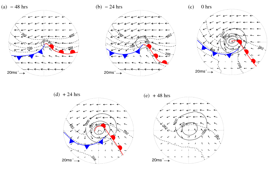
Horizontal composites at (a) 48 and (b) 24 hours before time of maximum intensity, (c) at the time of maximum intensity, and (d) 24 and (e) 48 hours after maximum intensity. Position of 925 hPa fronts; closed mslp contours (solid, at 10 hPa intervals); 925 hPa system relative wind vectors and 925 hPa θe (dashed, at 282, 290 and 298 K).