Assimilation of sources and sinks in 4d-Var

This page is under construction - 26/05/10

Introduction

Often in science important quantities are being studied that cannot be measured directly. The problem of determining the locations and strengths of sources and sinks of a trace gas in a domain is one example, which is investigated here.

The problem of estimating the source and sink field of a tracer in a fluid is studied here by developing and testing a dynamic data assimilation system that works with a fictious single-level global atmosphere. This atmosphere advects a tracer around the model's domain with known winds but with an unknown source/sink field which injects or removes tracer as time progresses.

The problem may be posed as follows. How is it possible to gain knowledge of this source/sink field given (i) sparse and imperfect observations of the tracer field over a time window and (ii) the imposed constraint that the tracer field itself evolves in time according to a tracer transport model? This problem is difficult to solve not least because only the tracer field itself (at sparse locations) is observed directly. There are no direct observations of the source/sink field - this field must be inferred using inverse techniques.

This is a nice example of an inverse problem. The solution to this inverse problem relies on a number of things.

• The existance of a soluble forward problem. Given a source/sink field (and initial conditions of the tracer), the forward problem predicts the observation values that would be recorded (give or take observation error) at prescribed locations and future times.
• That the source/sink field is observable. Even though it is not observed directly, this condition requires that there is enough information in the tracer observations to infer information about the source/sink.

Brief description of the set-up of our toy problem

In our toy problem, the atmosphere is 2-D (longitude/latitude) for simplicity and the source/sink field is taken to be constant over a 10-day assimilation window. The aim is to estimate the source/sink field (and simultaneously the tracer initial conditions) by assimilating a set of synthetic observations of the tracer only. The source/sink and initial tracer fields are assigned a-priori values, but we assume that no prior knowledge of the source/sink field is known (implemented by setting the source/sink a-priori to zero).

The forward model

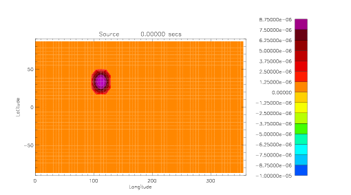
Suppose that the source/sink and initial tracer fields are known, e.g. the following fields.

The source/sink field: zero except for the region in the northern hemisphere which constantly injects tracer into the atmosphere.

The initial tracer field.

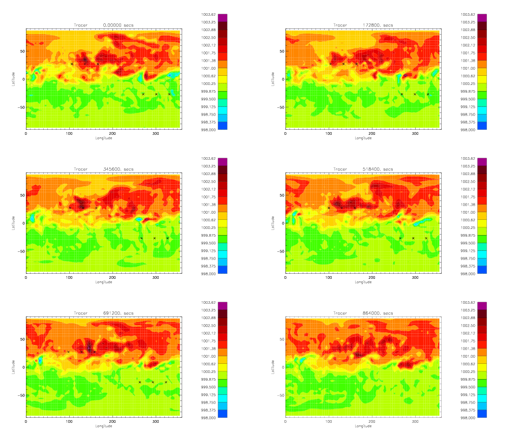
The forward model advects the initial conditions with prescribed winds with the injection of tracer at the source location.

Evolution of the tracer field over 10 days. The crosses denote the locations of observations. The animation will loop 100 times. Click SHIFT-RELOAD to start the looped animation again.

For our inverse problem experiments, first this run is made and taken as the 'truth' (or 'nature') state from which synthetic observations at selected positions and times (crosses in the above animation) by extrating the nature value at theses points and adding random noise extracted from a specified Gaussian distribution. For the purposes of testing the performance of the inverse problem the true source/sink and initial conditions are 'forgotten' in order to see how well they can be reconstructed from the observations.