Introduction
The purpose of this set of modules is to implement horizontal 1- and 2-dimensional spatial filtering of 2- and 3- dimensional output from MONC (and similar data), as well as 1D power spectra from 2D fields.
Filtering
This notionally corresponds to a split of a variable:

Note that this is not the same as coarse graining; the ‘resolved’ field  has the same number of gridpoints as the original, it is just smoother (with one exception noted below).
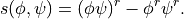
The code also produces ‘subfilter’ fluxes, variances and covariances: for any pair of variables  :
:
Power Spectra
The Power Spectra computed are conventional 2D power spectra averaged either in x- or y-direction, or radial spectra averaged around the azimuthal direction. Care has been taken to normalise in using standard and corrections can be applied to the radial spectra. See Durran et al. (2017) for details.
Output Files
An important feature of the code is that it creates two types of derived files.
A single file containing intermediate data such as
interpolated to the w grid, stored at variable th_L_on_w in NetCDF. This must be setup by the user using
subfilter.subfilter.setup_derived_data_file(). The user must tell the code to use it by setting options[‘save_all’] = ‘Yes’. The file name is created from arguments destdir, source_file and fname.A file for each filter containing filtered variables and sub-filter counterparts. This must be setup by the user using
subfilter.subfilter.setup_filtered_data_file(). The file name is created from arguments destdir, source_file, fname and filter_def.id.
Filters
- A number of filters have been implemented, currently
Gaussian.
Spectral wave cutoff.
Spectral cylindrical wave cutoff.
Running mean (or ‘top-hat’).
2D version of the 1-2-1 filter.
For completeness, a ‘whole domain’ filter in which the resolved field is the horizontal domain average. In this case the resolved field has no horizontal dimensions.
Input Transforms
Basic variables (‘u’, ‘v’, ‘w’, ‘th’, ‘p’, ‘q_vapour’, ‘q_cloud_liquid_mass’, ‘q_cloud_ice_mass’) are expected to be available in the input file. If MONC is used, the horizontal grid specification is corrected on input to ‘x_p’ or ‘x_u’, ‘y_p’ or ‘y_v’ as appropriate.
To facilitate use of other models, a list of aliases can be provided under the key ‘aliases’ to translate variable names.
In order to facilitate comparisons and products, tools have been coded (efficiently but not very elegantly) to transform data from different points on the C-grid. Thus, second order terms can be computed correctly on required points just by specifying the ouput grid.
A number of derived variables have been implemented that are calculated provided the required inputs are available. These are provided in the subfilter.thermodynamics.thermodynamics module.
Examples are:
‘th_L’ |
Liquid water potential temperature |
‘th_v’ |
Virtual potential temperature |
‘th_w’ |
Wet bulb potential temperature |
‘q_total’ |
Total water |
‘buoyancy’ |
|
 .
. .
. .
. ,
where the mean is the domain mean.
,
where the mean is the domain mean.While a variety of basic functions have been written, the intention is to use subfilter.subfilter.filter_variable_list() to automatically filter a list of NetCDF variables and write the output to a new NetCDF file,
and subfilter.subfilter.filter_variable_pair_list() to do the same with products of fields.
Each has a default list - this can easily be changed.
Todo
Code to calculate the deformation field and hence shear and vorticity has also been implemented but needs full integration.
Todo
The next step is to implement arbitrary derivatives, so one could specify in the variable list, e.g. “d_u_d_x_on_w”. This has been implemented in the trajectory code and will be ported to here for compatibility.
The subfilter.utils.difference_ops module now has general, grid-aware derivative and averaging functions.
These are used internally but the ability to use them in the input variable list has yet to be implemented, apart from some special variables like buoyancy gradient.
An example of use can be found in examples/subfilter_file.py.
Version History
Latest version is 0.5.0
New at 0.5
Complete re-structuring.
Addition of
subfilter.spectra.The
subfilter.subfilter.filtered_field_calc()function outputs filtered variables phi inder the names “f(phi)_r” and “f(phi)_s”.
New at 0.4
Use of xarray.
Use of dask for filtering.
Correction of MONC grid specifications on input.
New at 0.3
The filters.filter_2D class has been replaced with
subfilter.filters.Filter. This now accepts an optional argument ndim when creating a Filter instance. This may be 1 or 2 and defaults to 2. The use_ave option is no longer supported.The
subfilter.subfilter.filter_variable_pair_list()function outputs filtered pairs inder the name “s()_on_grid” where “grid” will be “u”, “v”, “w” or “p”.
New at 0.2
New ‘options’ dictionary passed to many functions.
- More efficient FFT convolutions. options[‘FFT_type’] can equal:
‘FFTconvolve’ for original implementation. Deprecated.
‘FFT’ for full FFT.
‘RFFT’ for real FFT.
- Two types of derived files are produced.
As before, a file for each filter containing filtered variables and sub-filter counterparts. This must now be setup by the user using
subfilter.setup_filtered_data_file().A single file containing intermediate data such as
interpolated to the w grid, variable th_L_on_w in NetCDF.
This must now be setup by the user using subfilter.setup_derived_data_file(). The user must tell the code to use it by setting options[‘save_all’] = ‘Yes’.