Proj1.5 Notebook
Tue Dec 20 11:47:07 GMT 2016
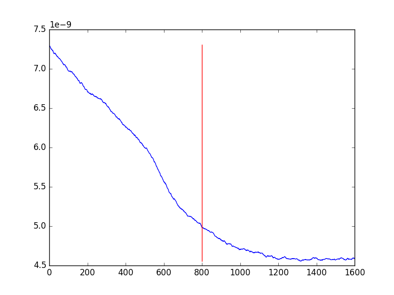
Spinup jobs (non-interactive ice/defined GrIs topog). Ice tile fractions are initialised as 10km of ice (i.e., snow at ice-density).
- xmvlf: CTL run. Present day SST/SICE.
- xmvlg: Perturbed. RCP4.5 SST/SICE from Jonathan.
Script: Annual 1.5m temp timeseries
import pylab as py
import sys
# Add to PYTHONPATH to make global:
sys.path.append('/DUM/DUM/Projects/FAMOUS/lib')

import umfile
import umfield

expid='xmvlf'
expid='xmvlg'

fpref='/DUM/DUM/Data/plane-01/DUM/FAMOUS/'+expid+'/'+expid+'a#pa00000'

marr=['ja','fb','mr','ar','my','jn','jl','ag','sp','ot','nv','dc']
stash=3236

#nyr=100

nyr=99 # As final year is missing Dec
yr1=1958

nmn=len(marr)


t15a=py.zeros(nyr,dtype='f8')

for yy in range(nyr):
 year=yr1+yy
 print year
 inf1=fpref+str(year)
 if yy == 0:
   infile=inf1+marr[0]+'+'
   hvals=umfield.get_pphead(infile)
   nx=hvals.ihead[0][18]
   ny=hvals.ihead[0][17]

 mdum=py.zeros([nmn,ny,nx],dtype='f8')
 for mm in range(nmn):
   infile=inf1+marr[mm]+'+'
   tarray=umfield.get_fieldob(infile,stash=stash)
   mdum[mm,:,:]=tarray.data

 t15a[yy]=mdum.mean()

py.save('t15m_'+expid+'_'+str(yr1),t15a)

py.figure(2)
py.clf()
py.plot(t15a)
py.title('t1.5 '+expid)
py.show()


#Tue Dec 20 17:06:37 GMT 2016
import pylab as py
import time
import sys

toc=273.15
ctl=py.load('t15m_xmvlf_1958.npy')
prt=py.load('t15m_xmvlg_1958.npy')

nt=ctl.size
dtime=py.arange(nt)+1958

tsr=(time.strftime("%d/%m/%Y %H:%M"))
fname=(sys.argv[0])
py.figure(10)
py.clf()
fig,ax=py.subplots()
ax.plot(dtime,ctl-toc,'r',linewidth=2,label='CTL (xmvlf)')
ax.plot(dtime,prt-toc,'b',linewidth=2,label='PRT (xmvlg)')
ax.legend()
ax.grid()
fig.text(0.8, 0.45, tsr,
         fontsize=40, color='gray',
                  ha='right', va='bottom', alpha=0.5)
fig.text(0.8, 0.55, fname,
         fontsize=40, color='gray',
                  ha='right', va='bottom', alpha=0.5)
py.xlim([1950,2060])
py.ylim([2,9])
py.title('Global Average 1.5m Temperature')
py.ylabel('Temp (C)')

py.show()

py.savefig('temp1.5m_both.png')
#Tue Dec 20 17:54:23 GMT 2016
Thu Dec 22 09:47:56 GMT 2016
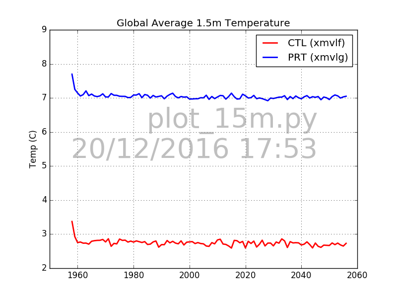
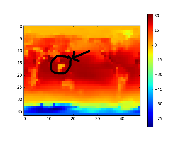
The diff(T_1.5m) between xmvlf and xmvlg is ~ 3.3K (the SSTs have a T_diff of ~ 2.2K).Found a problem with the SST infilling (for coastal tiling). Land mask was set to zero, and this was seeping through as a valid (fractional) surface temperature ... leading to cold spots in the Indian ocean. Tropical location had large weighting on global mean.
Script: SST infill
import pylab as py
import umfile
from copy import copy

# This does "MORE" infilling, wrt coastal tiling
# Originally from .../Projects/FAMOUS/Boundary

def box_av(inb,sw=0):
  nn=inb.size
  if nn != 9:
    print 'error'
    raise
  old=inb[1,1]
  inb=inb.reshape(9)
  ick=py.where(inb > -1000)[0]
  if len(ick) > 0:
    res=inb[ick].mean()
  else:
    if sw == 0:
       res=0
    else:
       res=old
  return res

def fill_in(inarr,sw=0):
  print 'fill',sw
  nn=inarr.shape
  nx=nn[1]
  ny=nn[0]
  nx2=nx+2
  temparr=py.zeros([ny,nx2],dtype=inarr.dtype)
  res=py.zeros([ny,nx],dtype=inarr.dtype)
  temparr[:,1:nx+1]=inarr
  temparr[:,0]=inarr[:,nx-1]
  temparr[:,nx2-1]=inarr[:,0]
  #print temparr[27,:]
  for yy in range (1,ny-1):
   for xx in range(1,nx2-1):
     if temparr[yy,xx] < -1000:
       bdat=temparr[yy-1:yy+2,xx-1:xx+2]
       res[yy,xx-1]=box_av(bdat,sw=sw)
     else:
       res[yy,xx-1]=temparr[yy,xx]
  res[0,:]=inarr[0,:]
  # Bodge
  res[ny-1,:]=inarr[ny-1,:]
  return res

# Suck in SST climatologies and pop them out again to cope with coastal tiling

infile='/DUM/DUM/Data/acacia-11/FAMOUS/ancil/qrclim.sst'
fbtype,idtype,rdtype,bits,bytes=umfile.ftype(infile)

fixhdr=umfile.get_fixhdr(infile,idtype)
intc,e1=umfile.get_const(infile,fixhdr,idtype,rdtype,bytes,field='intc')
realc,e2=umfile.get_const(infile,fixhdr,idtype,rdtype,bytes,field='realc')
ihead,ec=umfile.get_const(infile,fixhdr,idtype,rdtype,bytes,field='lookupi')
rhead,ed=umfile.get_const(infile,fixhdr,idtype,rdtype,bytes,field='lookupr')

nsh=ihead.shape
print nsh
np=nsh[0]

dstart=ihead[0,28]*8
offset=ihead[0,28]*8
dpack=ihead[0,29]

datao=py.zeros([np,dpack],dtype=rdtype)
for i in range(np):
  offset=ihead[i,28]*8
  dum=py.memmap(infile,dtype=rdtype,offset=offset,shape=dpack,mode='r')
  dum2=copy(dum)
  cum=dum2[0:1776].reshape(37,48)
  dfix1=fill_in(cum,sw=1)
  dfix=fill_in(dfix1,sw=1)
  dum2[0:1776]=dfix.reshape(37*48)
  datao[i,:]=dum2


fixhdr_new=py.copy(fixhdr)
### Write file
f=open('/DUM/DUM/Data/acacia-11/FAMOUS/ancil/qrclim.sst-FILL3','wb')
print f.tell()
f.write(fixhdr_new)
f.write(intc)
f.write(realc)
print f.tell(), (fixhdr_new[149]-1)*8
for i in range(np):
  f.write(ihead[i,:])
  f.write(rhead[i,:])
print f.tell(), (fixhdr_new[159]-1)*8, 'here and f159'
f.seek((ihead[0,28])*8,0)
print f.tell(), (ihead[0,28])*8, 'here again and ihead0,28'
for i in range(np):
  f.write(datao[i,:])


f.close()


#makesst1v3.py
#Thu Dec 22 09:57:50 GMT 2016
- xmvlf re-run submitted with corrected SST. Run so far indicates diff(T_1.5m) of ~ 2.75K. This equated to a Fettweis/SMB anomaly of 409 Gt.
- xmvlg extended: another 300 years submitted (previous runs suggest a 100-year snow spinup is not enough).
- Annual 1.5m temperatures Dec-to-Dec calculated (alternative to above).
New Runs:
- xmvlh: perturbed run with alternative (maybe warmer) SSTs from Jonathan (400 years).
- xmvli: perturbed run with alternative (maybe warmer) SSTs from Jonathan + perturbed CO2(400 years).
mix_ratio=(44/28.8) * (ppm_val/1000000)For 2100, and 4.5 W m-2 forcing ... CO2 is about 2.3 * preindustrial (2.3 * 280 = 644). So, 9.84e-4 kg/kg (xmvli)
Sat Dec 24 17:39:37 GMT 2016
xmvlf submitted for another 300 years.Tue Jan 3 15:28:22 GMT 2017
Problems
Early failures on runs. Assume disk space issues.- xmvlf: 2058-2182.
- xmvlg: 2058-2337.
- xmvlh: 1958-2212 (actually showing as still running at 12x100%. KILLED).
- xmvli: 1958-2211.
Attempted fix
Moved runs DATA_DIR to point to acacia-12 (from plane-01).- xmvlf: Restarted at 2182 for a 175 year run (complete).
- xmvlg: Restarted at 2337 for a 20 year run (complete).
- xmvlh: Restarted at 2212 for a 145 year run (complete).
- xmvli: Restarted at 2211 for a 146 year run (complete).
Wed Jan 4 10:10:34 GMT 2017
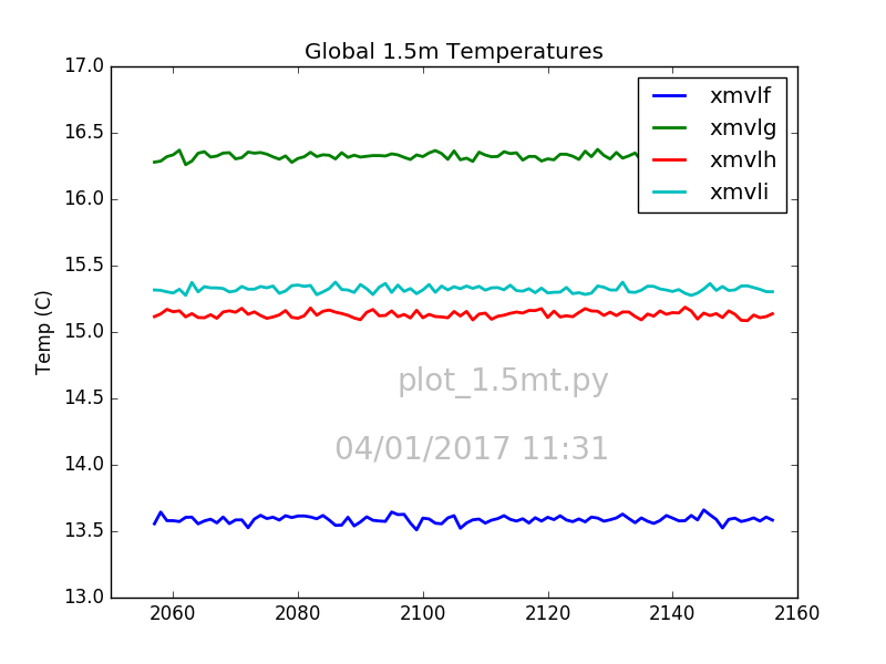
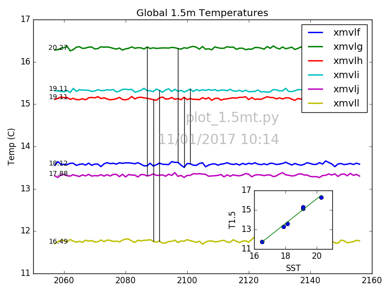
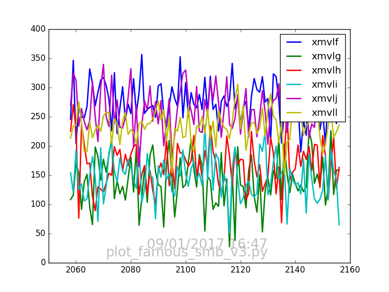
See above for run completion stats.Present output is ~0.7GB a model year (may need to trim the monthly output). Output from the second century of the runs: Figure: 1.5m temperature from simulations
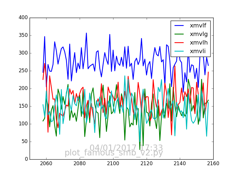
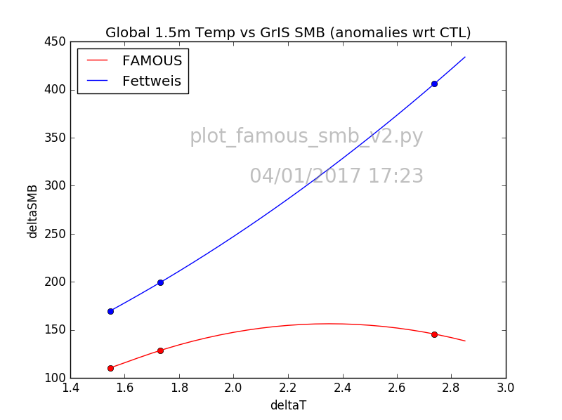
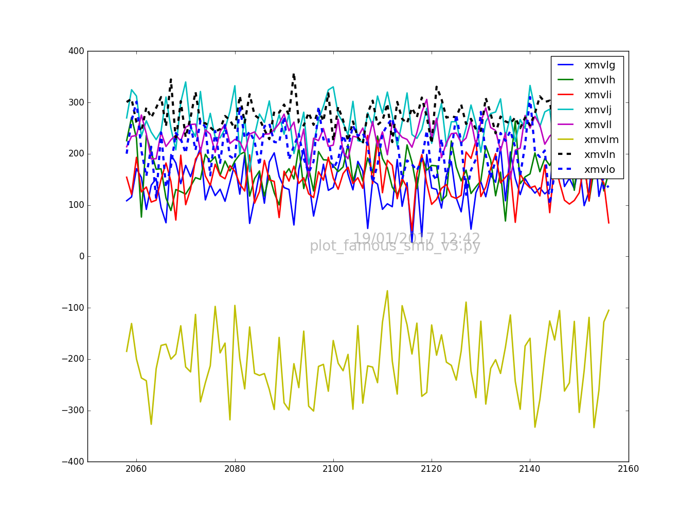
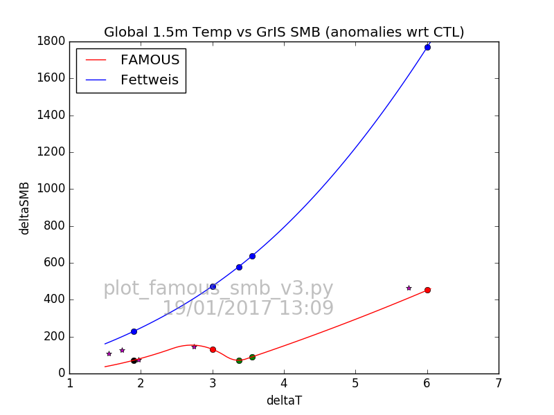
GrIS Surface Mass Balance (SMB) from model, compared with Fettweis value
These are 30-year averages, with t=0 150-years into run. Data are purely from FAMOUS (i.e., not downscaled in any way).| dTAS (K) | dSMB (GT/yr) | dSMB_f (GT/yr) | |
|---|---|---|---|
| xmvlg | 2.74 | 145.69 | 406.10 |
| xmvlh | 1.55 | 110.55 | 169.82 |
| xmvli | 1.73 | 128.65 | 199.43 |
Comparison of SST winter/summer forcing
Zero contour line in black.TODO: Check with ECMWF derived SST climatology.
Figure: Comparison of SST winter/summer forcing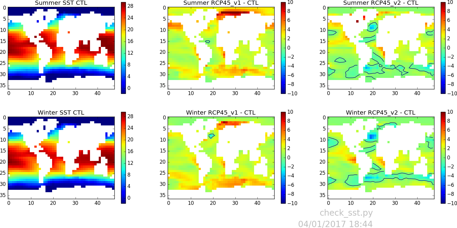
Thu Jan 5 12:19:06 GMT 2017
Additional meta-data:xlmvlf
SST Data/acacia-11/FAMOUS/ancil/qrclim.sst-FILL3
SIC Data/acacia-11/FAMOUS/ancil/qrclim.ice-FILL
xmvlg
SST jonathan/ancil/sst_FAMOUS_HadGEM2-ES_rcp45_2280-2299.anc
SIC jonathan/ancil/sic_FAMOUS_HadGEM2-ES_rcp45_2280-2299.anc
xmvlh/xmvli
SST jonathan/sst_FAMOUS_IPSL-CM5A-LR_rcp45_2180-2200.anc
SIC jonathan/sic_FAMOUS_IPSL-CM5A-LR_rcp45_2180-2200.anc
Fri Jan 6 15:34:01 GMT 2017
Additional control runs, model CTL SST/SIC forcing.xmvlj
CTL version of xmvlg.SST jonathan/ancil/sst_FAMOUS_HadGEM2-ES_piControl_2280-2299.anc SIC jonathan/ancil/sic_FAMOUS_HadGEM2-ES_piControl_2280-2299.anc
xmvll
CTL version of xmvlh/i. Info on IPSL-CM5A.SST jonathan/ancil/sst_FAMOUS_IPSL-CM5A-LR_piControl_2181-2200.anc SIC jonathan/ancil/sic_FAMOUS_IPSL-CM5A-LR_piControl_2181-2200.anc
Mon Jan 9 15:15:46 GMT 2017
Disk space issues again (over weekend). This time $HOME. Part resubmission required.- xmvlj: 200 year run (complete).
- xmvll: 200 year run (complete).
Tue Jan 10 12:17:31 GMT 2017
| Global seasonal mean SST (C) | ||
|---|---|---|
| Summer | Winter | |
| CTL1 (xlmvlf) | 17.94 | 18.09 |
| RCP45_v1 (xmvlg) | 20.11 | 20.24 |
| RCP45_v2 (xmvlh/i) | 18.94 | 19.03 |
| CTL2 (xlmvj) | 17.68 | 17.85 |
| CTL3 (xlmvl) | 16.27 | 16.41 |
Wed Jan 11 15:53:13 GMT 2017
MARV interranual SMB variabilityThu Jan 12 10:48:12 GMT 2017
Looking at the accumulation/ablation characteristics of the model. Figure: Accumulation/ablation
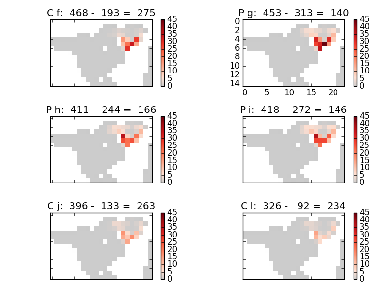
- SP Solid precip (snow): GrIS sum = 468 Gt
- SMB: GrIS sum = 275 Gt.
- AB Difference (ablation/melt): GrIS sum = 193 Gt. These are also the mapped values.
xmvlg (PERT) vs. xmvlj (CTL)
- dSP = 453 - 396 = 57 Gt (increase in precip)
- dSIMB = 140 - 263 = -123 Gt (decrease in accumulation)
- dAB = 313 - 133 = 180 Gt (increase in ablation/melt)
xmvi (PERT) vs. xlmvl (CTL)
- dSP = 418 - 326 = 92 Gt (increase in precip)
- dSIMB = 146 - 234 = -88 Gt (decrease in accumulation)
- dAB = 272 - 92 = 180 Gt (increase in ablation/melt)
mon Jan 16 12:00:00 GMT 2017
There are no direct tile albedo diagnostics.
Working on a calculation of albedo (α) using grain size.
From Kuipers(2011),
and using a simplified form of equation (4) (defined in equation (5)).
α = 1.48-(1.27048 * r**0.07)
Tue Jan 17 15:08:43 GMT 2017
Calculating albedo from SW components. Short runs needed, as:1| 1 | 3 | 335 |NET DOWN SURFACE SW FLUX ON TILESnot including in original STASH setup.
Short runs, for all configurations; started at 2157, 30-years in length (acacia-12).
- xmvlf: 2157, 30-years completed
- xmvlg: 2157, 30-years completed
- xmvlh: 2157, 30-years completed
- xmvli: 2157, 30-years completed
- xmvlj: 2157, 30-years completed
- xmvll: 2157, 30-years completed
New Simulations
xmvlm 4xCO2 boundary conditions. xlmvj is the CTL.CO2 mixing rato of 24.4e-04 kg/kg. (4*6.1e-04).
SST jonathan/ancil/sst_FAMOUS_HadGEM2-ES_abrupt4xCO2_1989-2008.anc
SIC jonathan/ancil/sic_FAMOUS_HadGEM2-ES_abrupt4xCO2_1989-2008.anc
xmvln MIROC5 boundary conditions: CTL simulation.
SST jonathan/ancil/sst_FAMOUS_MIROC5_historical_1980-1999.anc
SIC jonathan/ancil/sic_FAMOUS_MIROC5_historical_1980-1999.anc
xmvlo MIROC5 boundary conditions: PERT RCP45 simulation.
CO2 mixing rato of 9.84e-4 kg/kg (2.3 * preindustrial)
SST jonathan/ancil/sst_FAMOUS_MIROC5_rcp45_2081-2100.anc
SIC jonathan/ancil/sic_FAMOUS_MIROC5_rcp45_2081-2100.anc
Runs:
- xmvlm: 1957, 200-years submitted UM2
- xmvln: 1957, 200-years submitted UM2
- xmvlo: 1957, 200-years submitted UM2
Wed Jan 18 17:27:37 GMT 2017
Figure: Albedo PERT vs CTL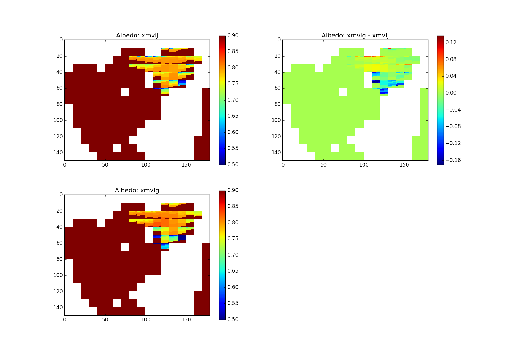
Thu Jan 19 11:55:14 GMT 2017
Note: Delicate balance between temperature and accumulation. CTL xmvlf has a bigger GrIS SMB (275 Gt/yr) than CTL xmvlj (263 Gt/yr). But, the latter is globally cooler. So dSMB (xmvlg vs. xmvlf) is greater than dSMB (xmvlg vs. xmvlj), though the dTAS is smaller. This is also seen in IPSL boundary simulations. The CTL xlmvl has a cold world starting point. Figure: 1.5m temperature from simulations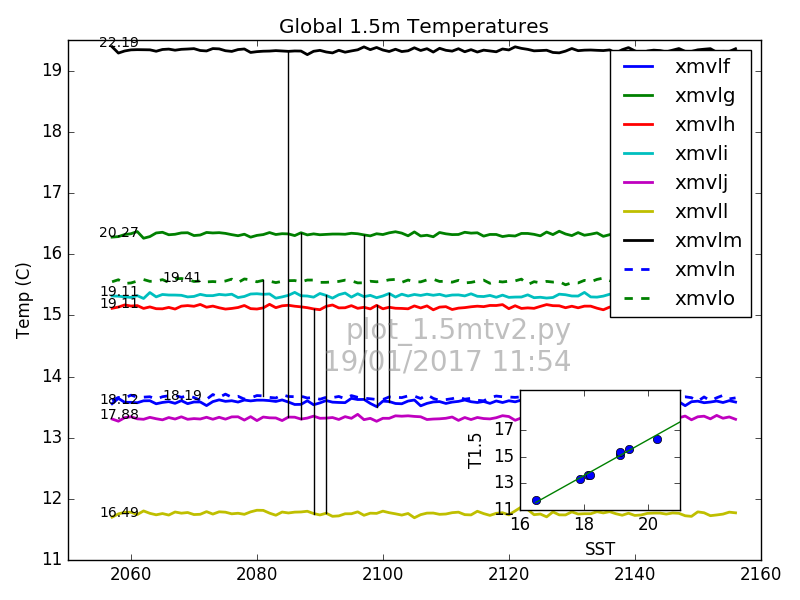
Wed Jan 25 11:17:51 GMT 2017
FAMOUS snow to bare ice transition: once snow density > 800 kg/m^3, surface is assumed to be bare ice with an albedo which has a linear dependence on temperature. Code lifted from tilealb.f:
             IF (gbm_rho_snow(l) .GT. 600.0)
    &             fsnow(l) = 1.0 - ((gbm_rho_snow(l)
    &                                       - 600.0) / 200.0)
             fsnow(l) = MIN(fsnow(l), 1.0)
             fsnow(l) = MAX(fsnow(l), 0.0)

               ALB_TYPE(L,N,BAND) = FSNOW(L)*ALB_SNOW(L,N,BAND) +
     &                          (1. - FSNOW(L))*ALB_TYPE(L,N,BAND)

!!! Thus, at gbm_rho_snow=800, ALB_TYPE ignores any ALB_SNOW contribution
!!! Reverts to bare ice, with a starting albedo of 0.78, which is adjusted
!!! wrt to the tile temperature
        TM=273.15
        aicemax(1) = 0.78
        daice(1) = -0.075

        alb_type(l,n,1) = aicemax(1)

        IF (tstar_tile(l,ntiles-nelev+k) .GT. (tm - 1.0)) THEN
          dt = tstar_tile(l,ntiles-nelev+k) - (tm - 1.0)
          alb_type(l,n,1) = aicemax(1) + (dt * daice(1))
Now, calculating the bare-ice temperature/albedo relationship offline.
Note: Using 1.5m temp, rather that Tstar.
Figure: FAMOUS bare ice temp vs albedo
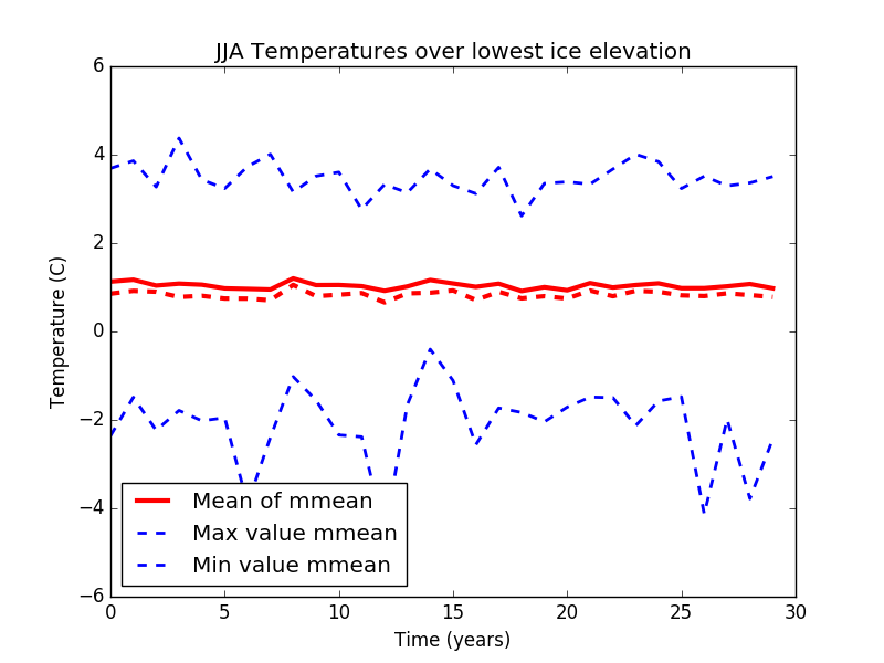
Lowest ice-elevation area > 4C  1.76376007122 %
Lowest ice-elevation area 3-4C  11.5015728019 %
Lowest ice-elevation area 2-3C  32.1883520289 %
Lowest ice-elevation area 1-2C  54.546315098 %
Percentage check... 100.0
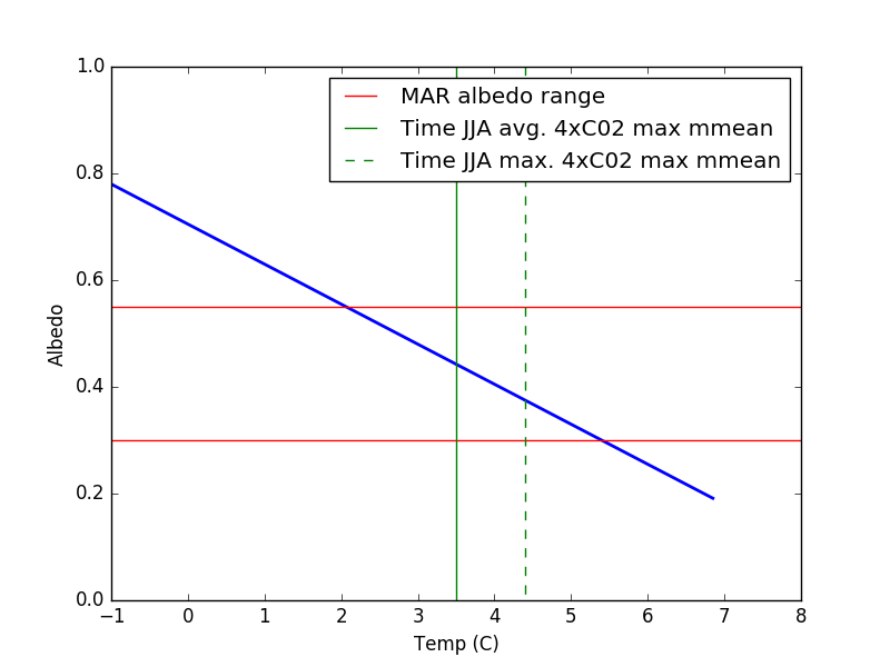
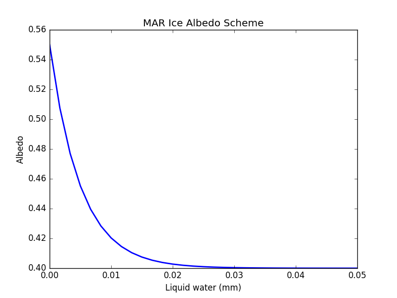
MAR Ice Albedo
From Tedesco(2017), the MAR bare-ice albedo is defined as:albedo = albedo_min + (albedo_max - albedo_min) * exp(-M * K) albedo_min,albedo_max - variable. In this paper set to 0.4,0.55 (elsewhere 0.3,0.55) K - scaling factor (200 kg/m^2) M - time-dependent accumulated excess surface meltwater before runoff (kg/m^2).Figure: MAR bare-ice albedo scheme
FAMOUS Refreeze
Initial calculation of refreeze (4xCO2 run).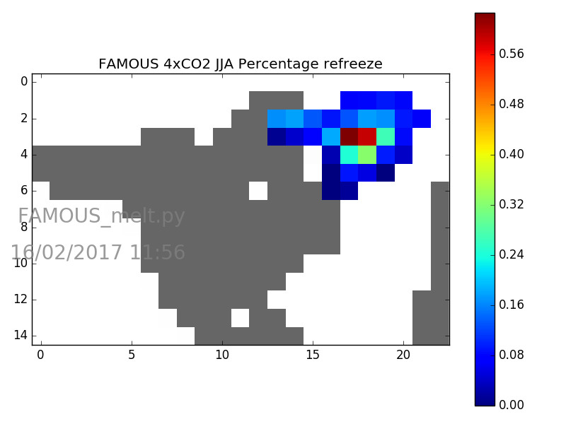
Fri Jan 27 14:38:02 GMT 2017
Note: FAMOUS percentage refreeze plot (above) has been replaced. Now the ratio of STASH8391/(STASH8391+STASH8237).Tue Jan 31 09:44:07 GMT 2017
Note: The near-IR SW is more important than than the visible spectrum wrt ice-radiation absorption. Figure: FAMOUS SW spectral split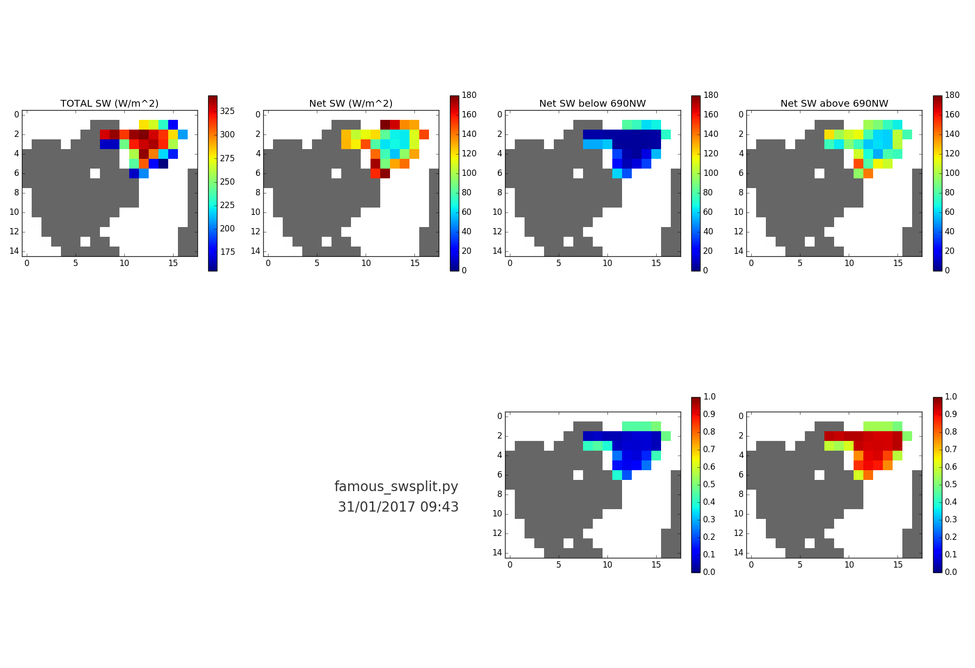
Mon Feb 6 16:00:30 GMT 2017
Following up on Equ (1) and (2) in Fettweis, FAMOUS has a linear relationship betweem the local JJA 600hPa temperature and global annual average at surface. Figure: FAMOUS Global vs regional/seasonal temps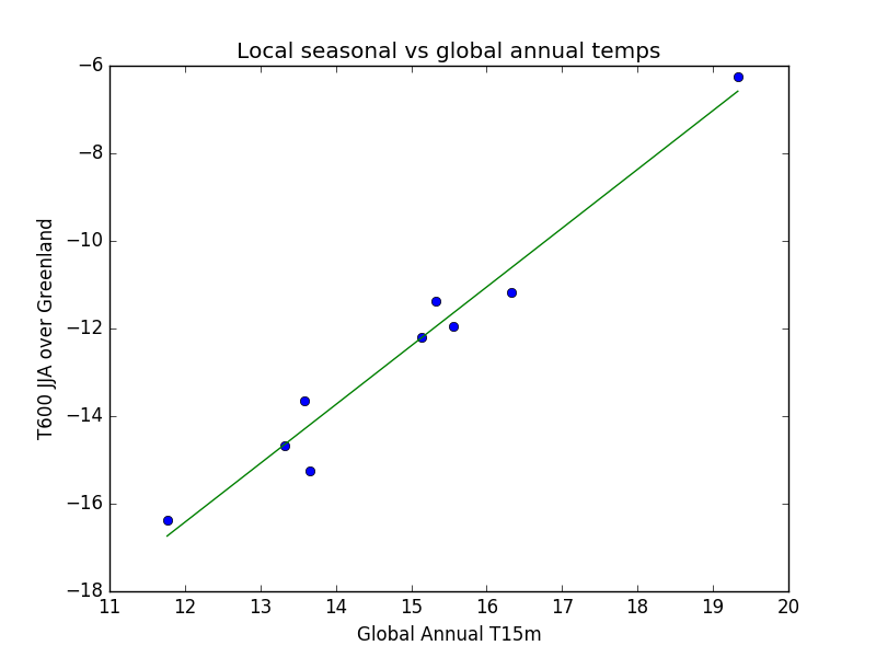
Thu Feb 16 10:27:47 GMT 2017
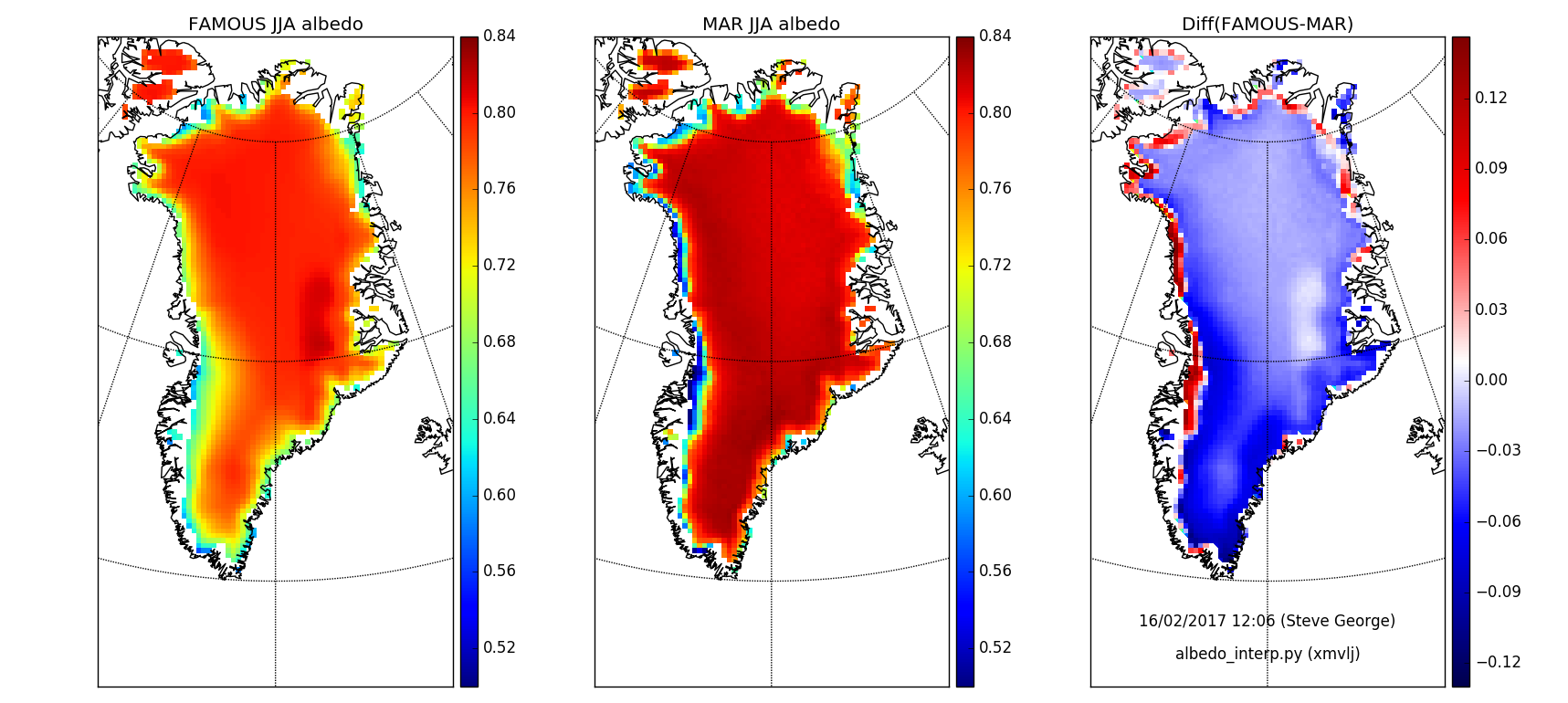
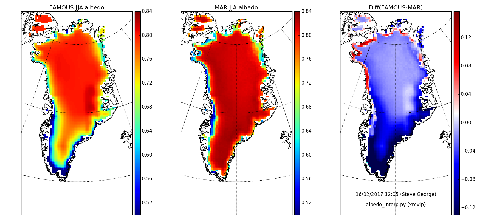
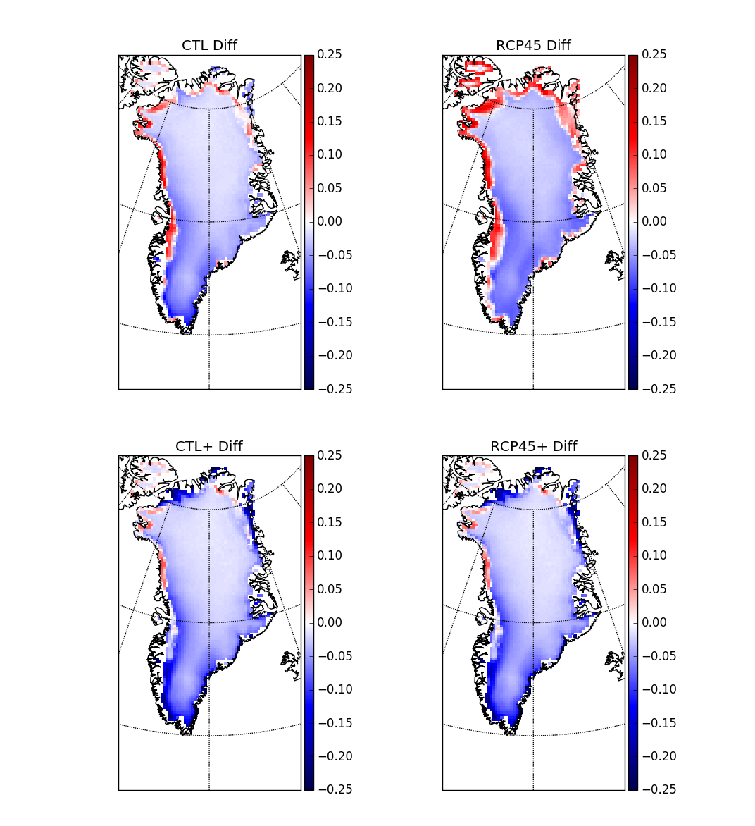
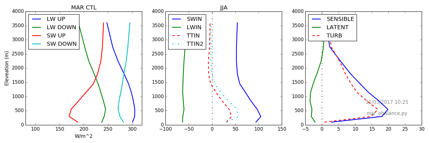
Comparing FAMOUS CTL (xmvlj) to MAR CTL simulation (30-years of FAMOUS).stash1235 - TOTAL DOWNWARD SURFACE SW FLUX stash3335 - NET DOWN SURFACE SW FLUX ON TILES albedo = 1.0 - (stash3335/stash1235)
From the regridded FAMOUS data
Maximum albedo: FAMOUS(0.82), MAR(0.83)Minmum albedo: FAMOUS(0.57), MAR(0.48) Figure: FAMOUS/MAR albedo
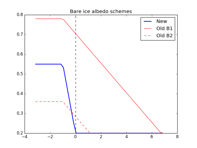
- xmvlp: copy of xmvlf, but with adjusted bare-ice characteristics.
tilealb.f

aicemax(1) = 0.55   # Previously  0.78
aicemax(2) = 0.55   # Previously 0.36
daice(1) = -0.35    # Previously -0.075
daice(2) = -0.35    # Previously -0.075

# Minimum albedo allowed 0.2
Albedo schemes plot. Note, surface temp of ice will not exceed 0C, so 'Old B1/B2' will have a min of ~ 0.7/0.28.
 Minmum albedo: FAMOUS(0.27), MAR(0.48)
Figure: FAMOUS/MAR albedo
Minmum albedo: FAMOUS(0.27), MAR(0.48)
Figure: FAMOUS/MAR albedo
Meeting 16-Feb-2017: notes
New Runs
FAMOUS/MIROC CTL had defective 3335 diagnostic output. Rerun for 30 years from 2057.- xmvln: MIROC5 CTL forcing for MAR comparison. 30-year run from 2057 started on um2. Complete
Fri Feb 17 17:27:59 GMT 2017
To be consistent, run 30-years from 2157.- xmvln: MIROC5 CTL forcing for MAR comparison. 30-year run from 2157 started on um2.
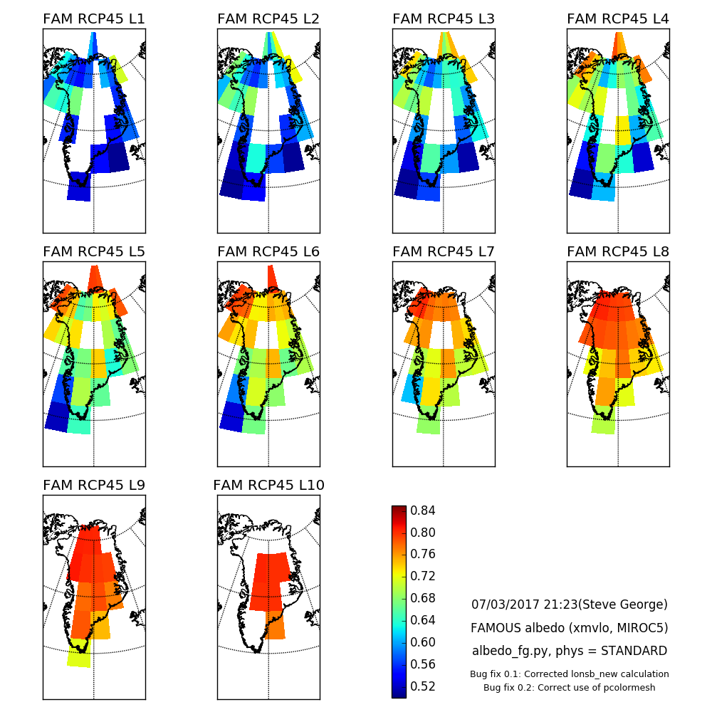
- xmvlo: MIROC5 RCP45 forcing for MAR comparison. 30-year run from 2157 started on um2.
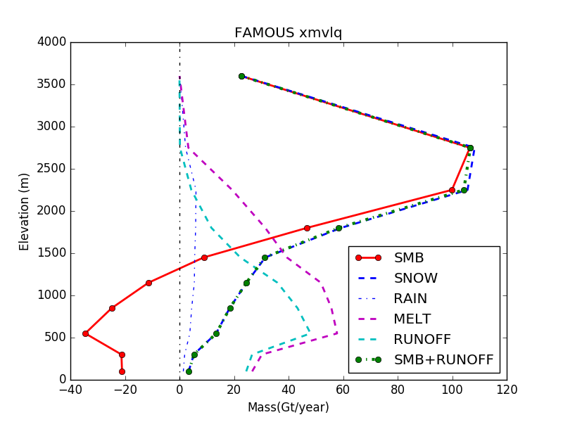
- xmvlq: MIROC5 CTL forcing for MAR comparison with new bare-ice albedo. 30-year run from 2157 started on um2.
- xmvlr: MIROC5 RCP45 forcing for MAR comparison with new bare-ice albedo. 30-year run from 2157 started on um2.
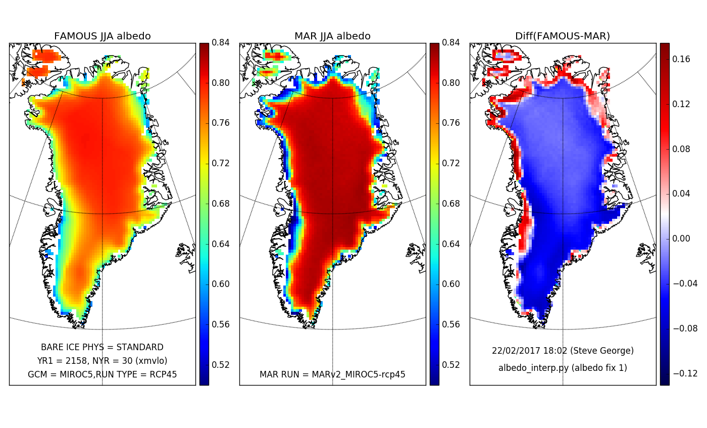
Mon Feb 20 17:07:54 GMT 2017
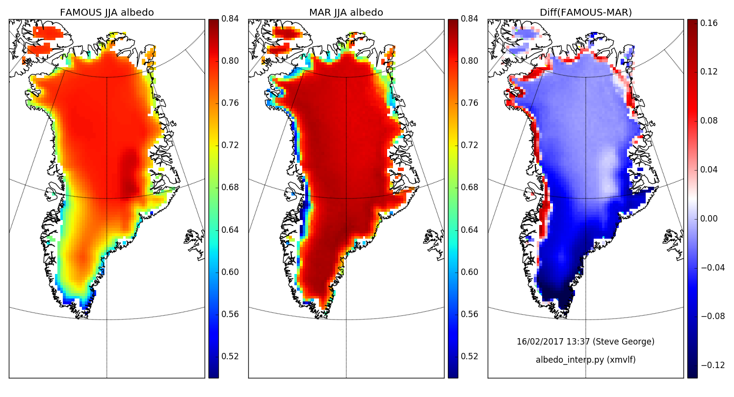
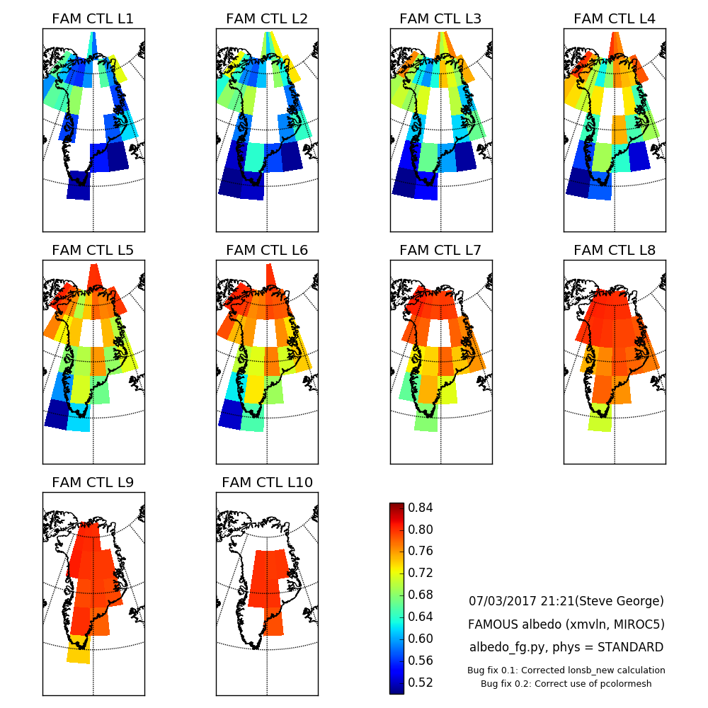
FAMOUS with MIROC5 SST/SIC forcing (as per MAR). Figure: FAMOUS/MAR albedo CTL STANDARD ICEWed Feb 22 18:05:11 GMT 2017
FAMOUS with MIROC5 SST/SIC forcing (as per MAR). Plot updates. Anomalous high albedo in previous plots. Tiles with small ice fraction (<0.001) seem to be ignored by the radiations scheme. This led to albedo values of 1.0 where net SW was zero (on a tile). Figure: FAMOUS/MAR albedo CTL STANDARD ICE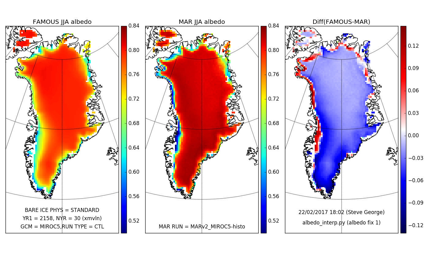
- xmvls: MIROC5 CTL forcing for MAR comparison with new bare-ice albedo. Also max albedo of fresh snow in IR band changed from 0.7 to 0.98. 30-year run from 2157 started on um2.
Thu Feb 23 10:35:28 GMT 2017
A bit to far on the albedo max! Figure: FAMOUS/MAR albedo CTL STANDARD ICE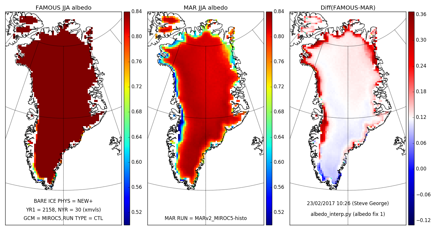
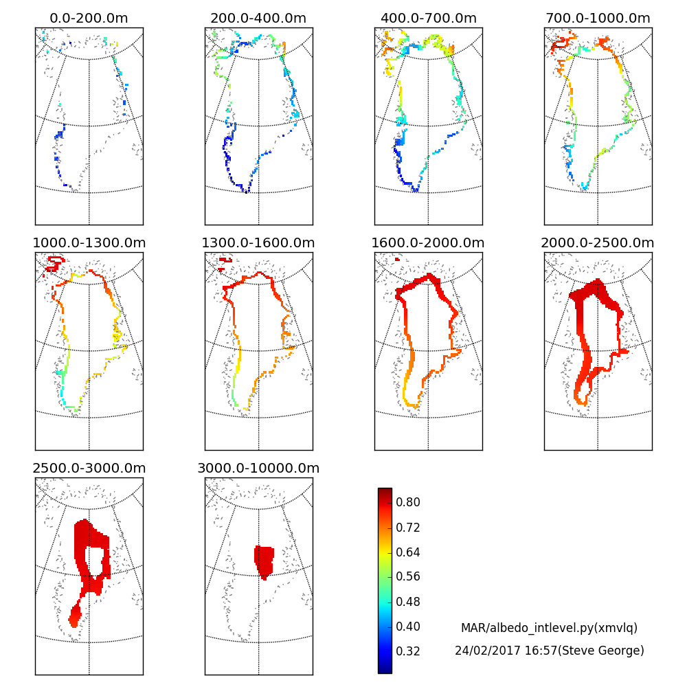
Fri Feb 24 17:00:55 GMT 2017
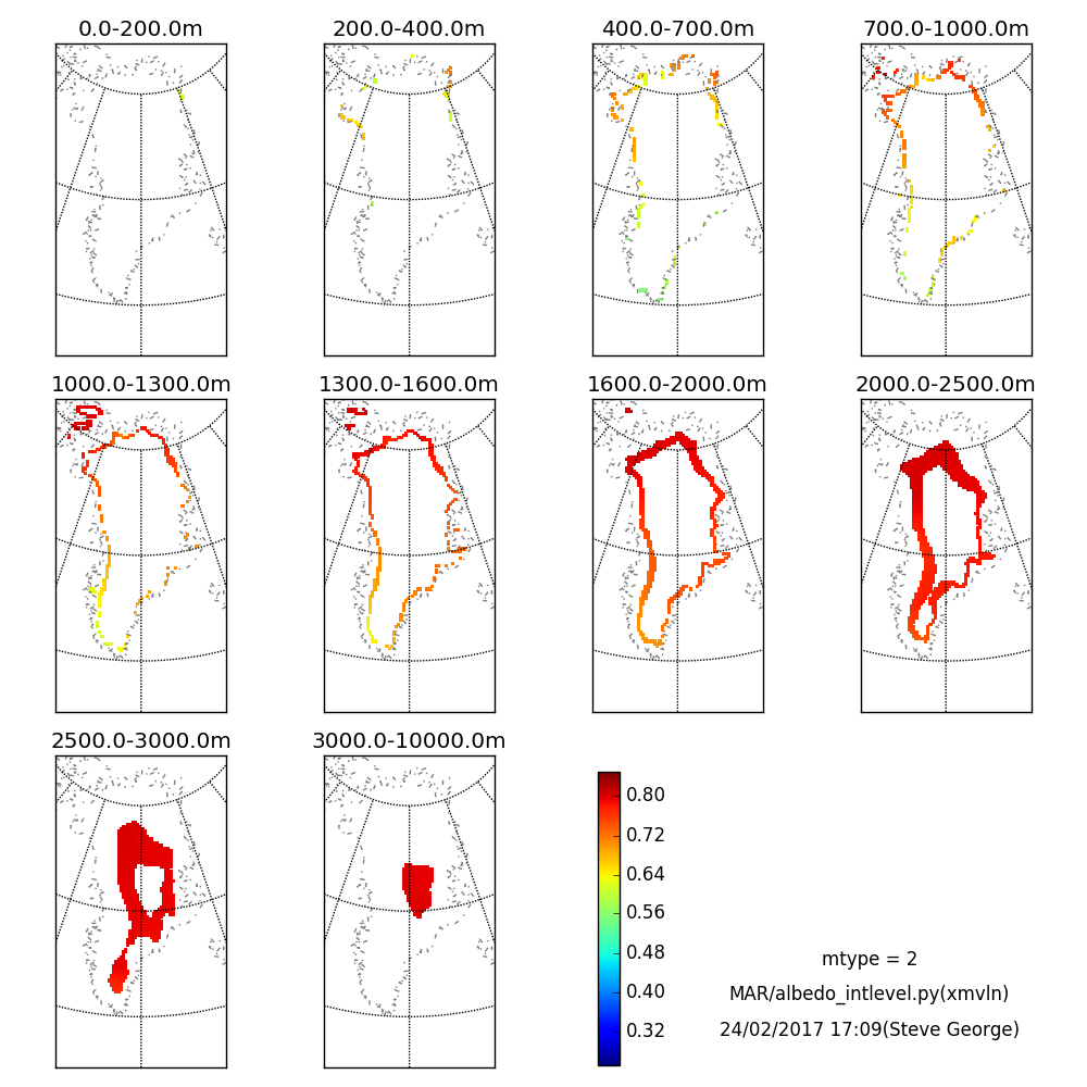
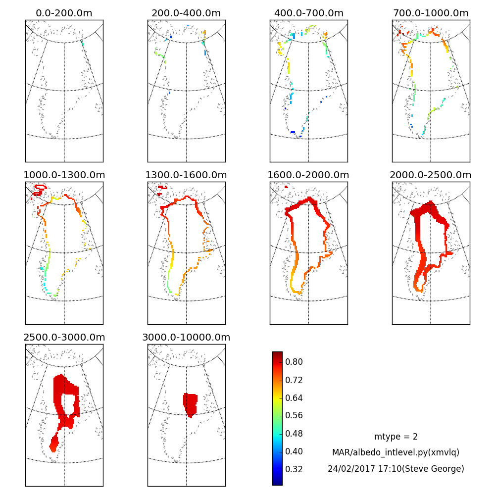
Albedo on each FAMOUS elevation class interpolated onto MAR topography. Following include tundra (non-ice points, mask=1) plus ice (mask=2). Figure: Albedo interp (xmvln)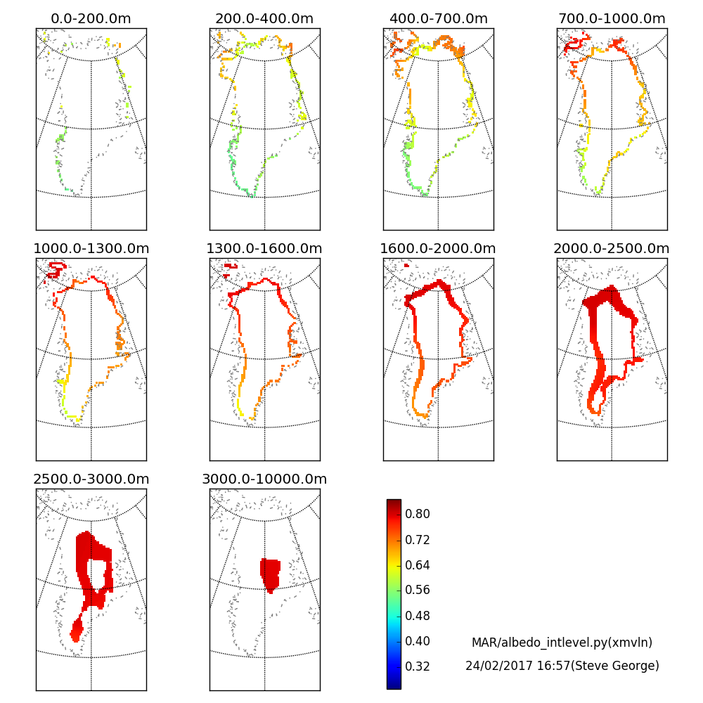
Fri Mar 3 19:35:49 GMT 2017
Regridding the high-res 2D MAR albedo field onto the FAMOUS 3D grid (with elevation classes).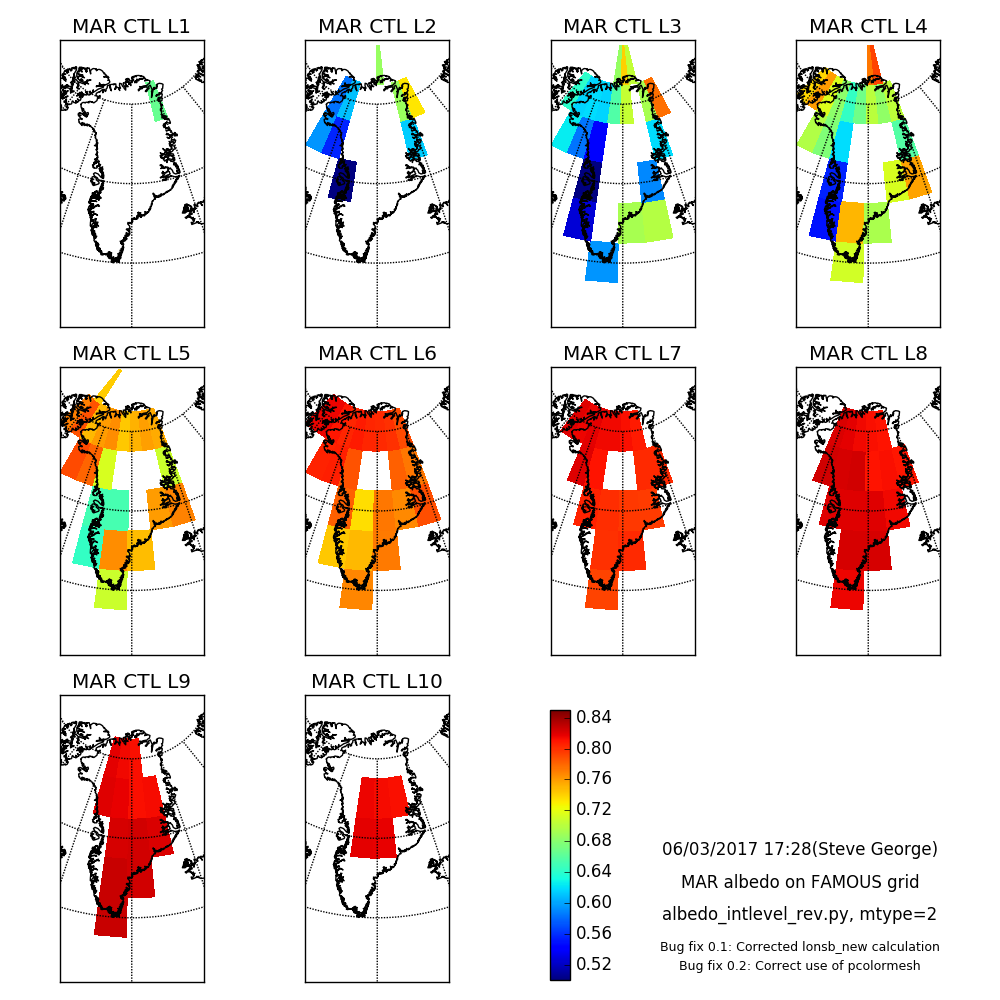
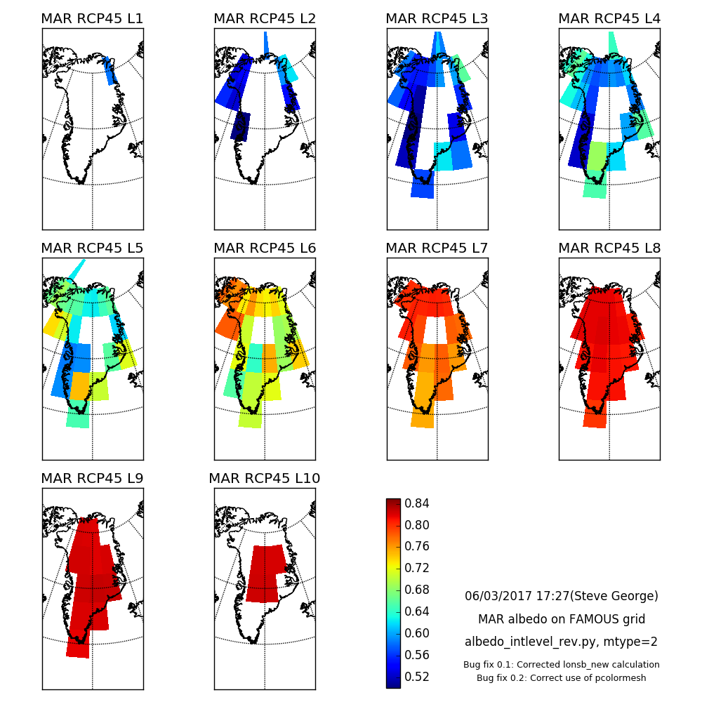
Mon Mar 6 17:30:03 GMT 2017
A couple of bug fixes in the MAR to FAMOUS algorithm. Plots above updated to new versions.Tue Mar 7 21:17:46 GMT 2017
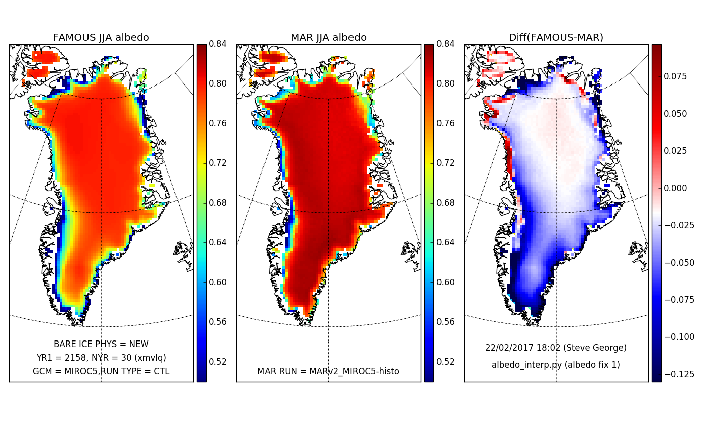
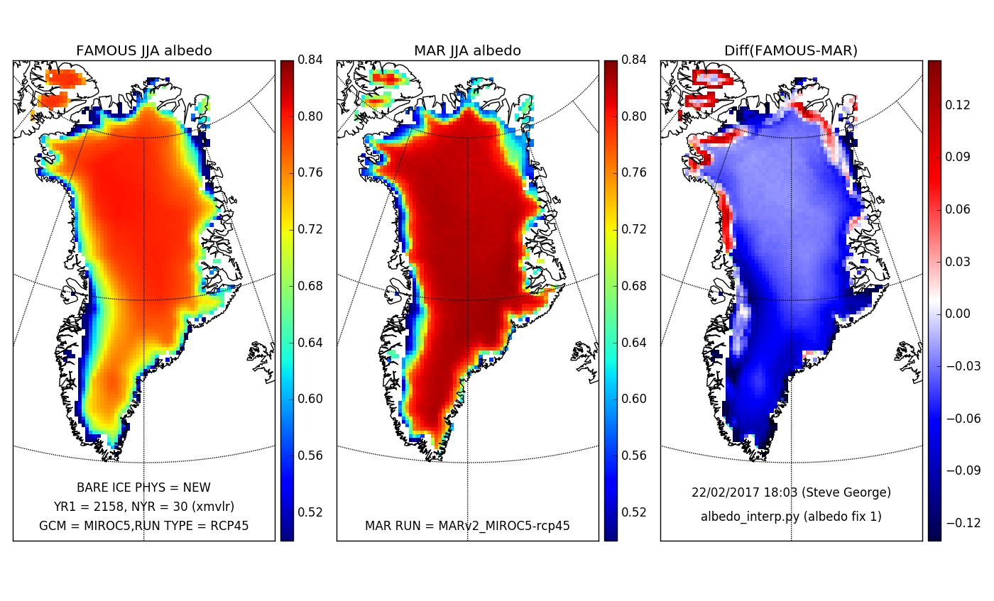
FAMOUS albedo on same grid as above (big fixes from earlier plots). Figure: FAMOUS new phys albedo CTL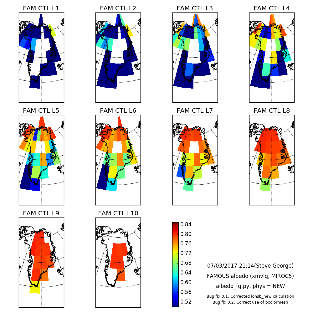
Wed Mar 8 16:24:32 GMT 2017
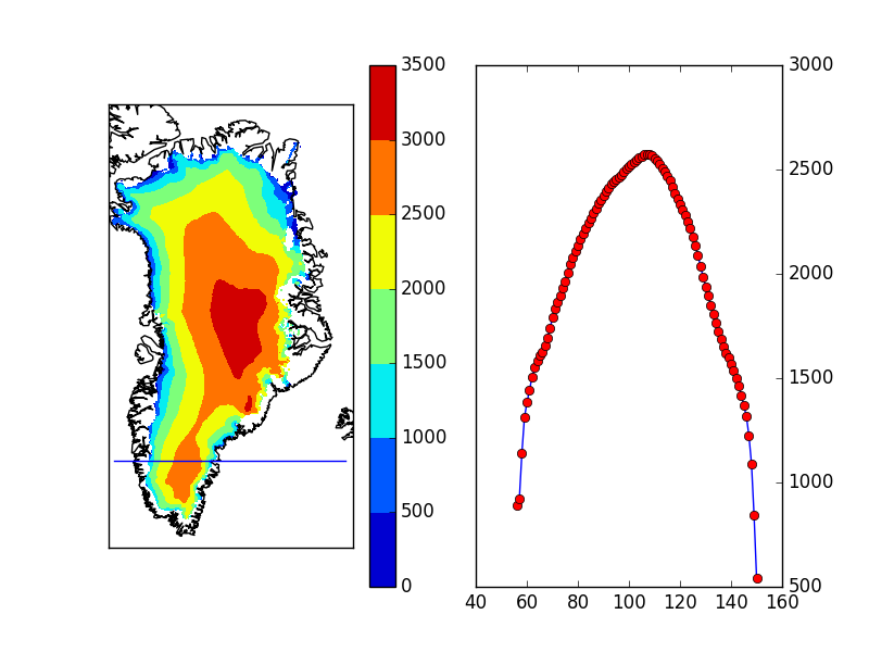
FAMOUS shows low-level ice fraction (i.e. 200-400m) on the SW coast ... and MAR not. Looking at cross sections from MAR and observations (5km resolution). Figure: MAR height cross section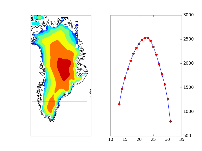
Thu Mar 9 15:21:25 GMT 2017
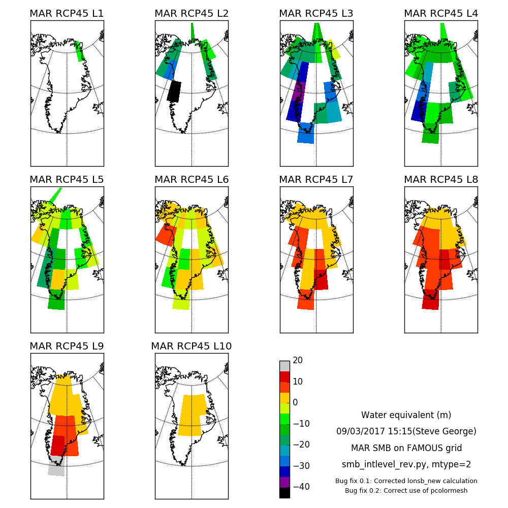
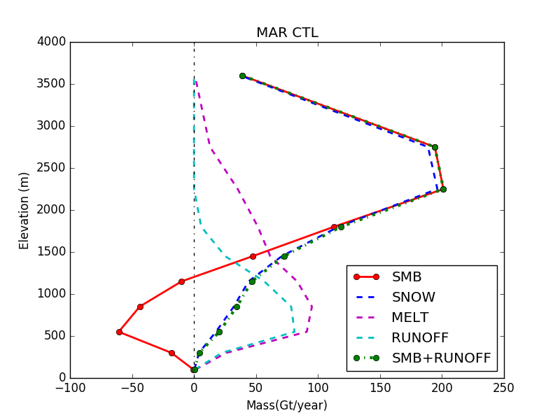
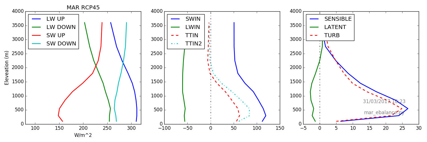
MAR SMB on FAMOUS levels. Figure: MAR F-SMB CTL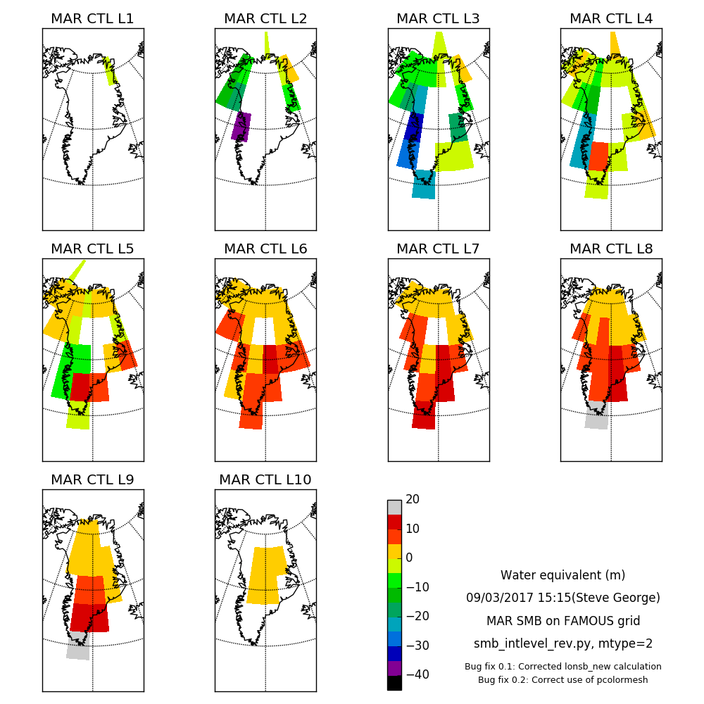
Mon Mar 20 17:28:42 GMT 2017
SMB with elevation. Figure: FAM vs. MAR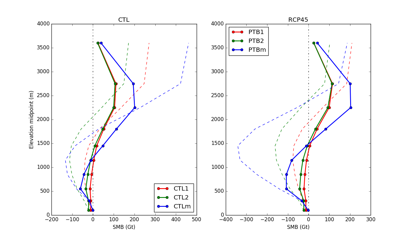
Tue Mar 21 14:02:48 GMT 2017
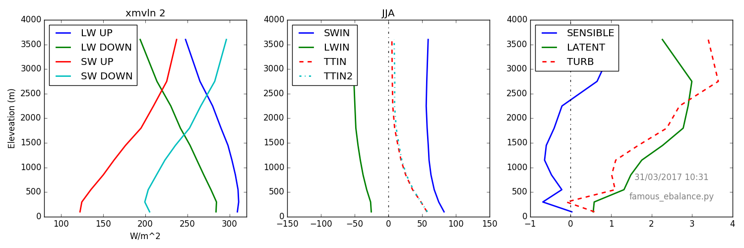
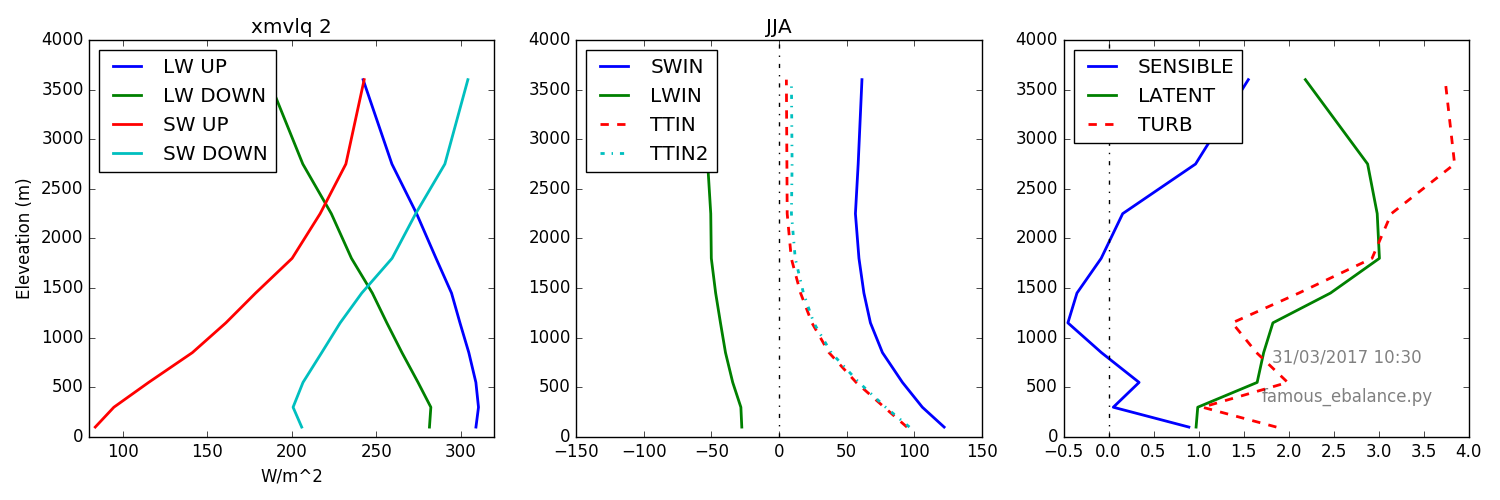
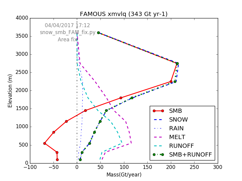
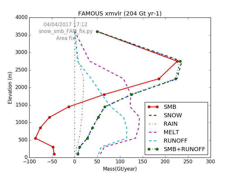
FAMOUS SMB components (CTL old/new physics) Figure: FAMOUS CTL (xmvln) SMB components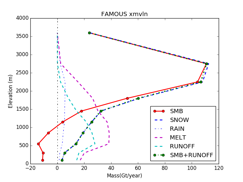
Mon Mar 27 18:00:57 BST 2017
For the surface energy calculations I need latent and sensible (on tiles). Run each simulation for another 10-years to get these.- xmvln: MIROC5 CTL forcing for MAR comparison. 10-year run from 2187 started on um2.
- xmvlo: MIROC5 RCP45 forcing for MAR comparison. 10-year run from 2187 started on um2.
- xmvlq: MIROC5 CTL forcing for MAR comparison with new bare-ice albedo. 10-year run from 2187 started on um2.
- xmvlr: MIROC5 RCP45 forcing for MAR comparison with new bare-ice albedo. 10-year run from 2187 started on um2.
Tue Mar 28 15:09:57 BST 2017
Above run again with the addition of the following diagnostics.3314 Surface net radiation on tiles 3316 Surface temperture on tiles
Thu Mar 30 15:06:43 BST 2017
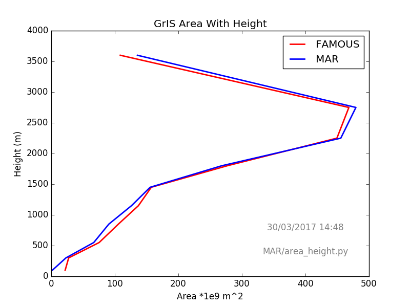
Comparison of ice-area in each elevation class.Note: Correction of area calculation in fammisc.py. Figure: GrIS area with height
Fri Mar 31 10:31:45 BST 2017
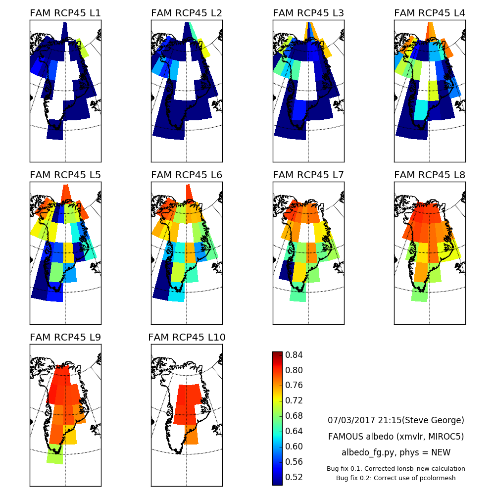
As above, but for perturbed (RCP45 MIROC5) runs. Figure: FAMOUS RCP45 (xmvlo)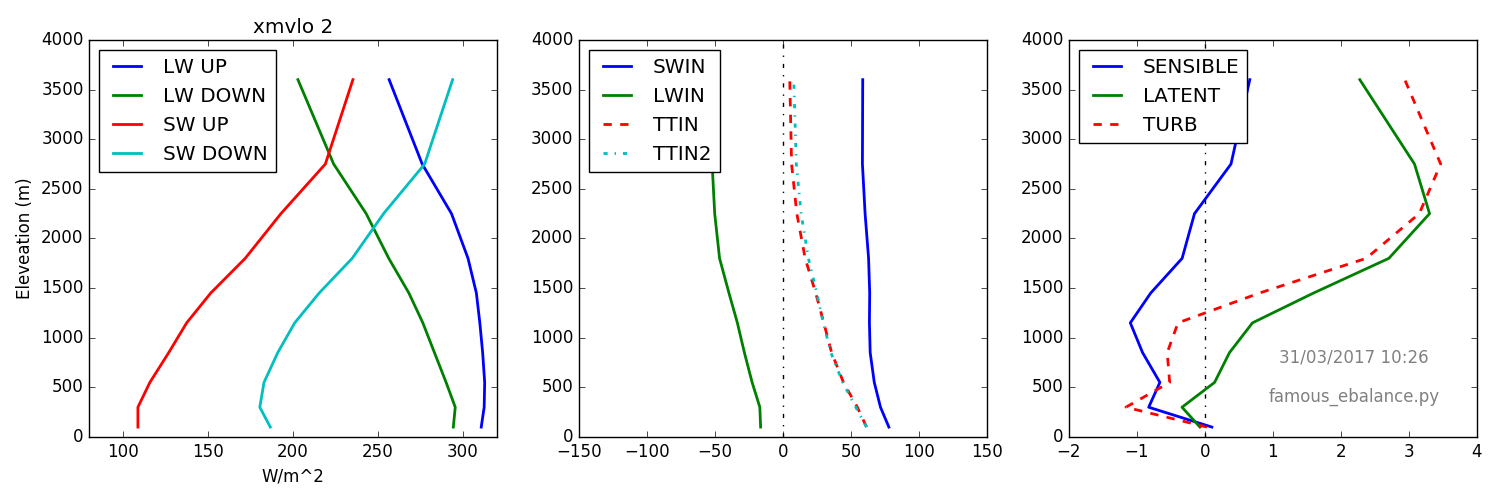
Thu Apr 6 10:08:44 BST 2017
MAR related changes
Introduced a threshold minimum wrt how many MAR boxes are required to create a FAMOUS box average (set to 4). Figure: MAR contribution to FAMOUS lev1 box average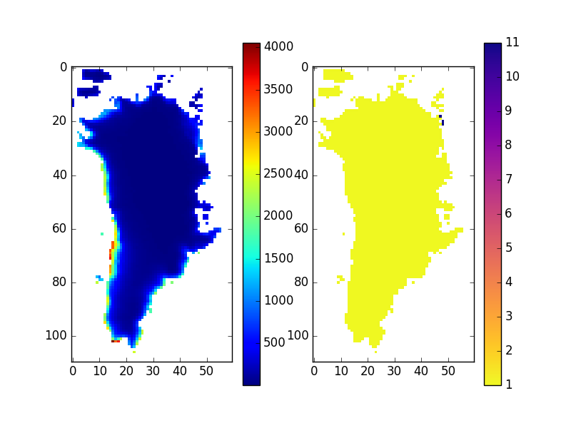

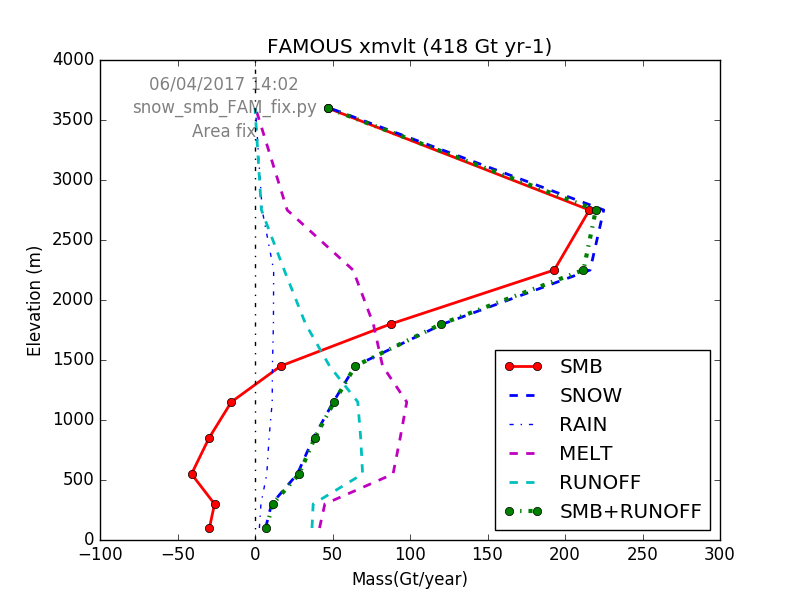
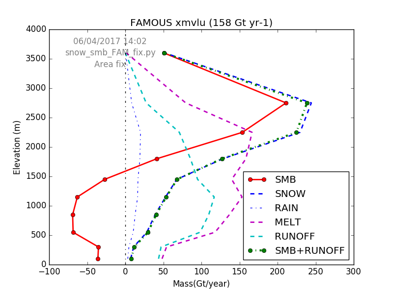
FAMOUS analysis
New height/mass balance calculations using fixed fammisc.py area calc. Figure: Mass/elevations averages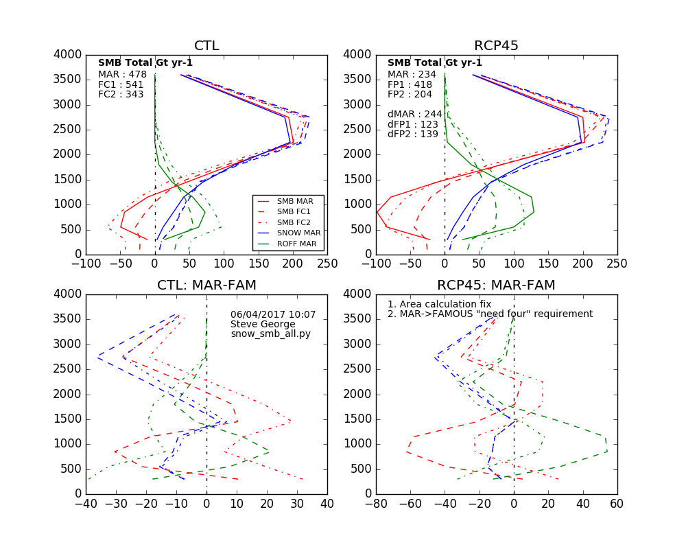
!+ seg 4/2017
! Calculated version:
!        tgrad=(t(i,BL_LEVELS)-t(i,1))/bldepth
!
! Use fixed temperature lapse rate
! What to use?
!     DALR ~ 0.0098 deg/m  (9.8 deg/km)
! Model:
!     LAPSE=0.0065     !  NEAR SURFACE LAPSE RATE
!     LAPSE_TROP=0.003 !  TROPOPAUSE LAPSE RATE
! Set to latter
        tgrad=0.003
!- seg
New runs with lapse rate change. From 2157 (30-years).
- xmvlt: As xmvlq, but with fixed temperature lapse rate for elevation calc.
- xmvlu: As xmvlr, but with fixed temperature lapse rate for elevation calc.
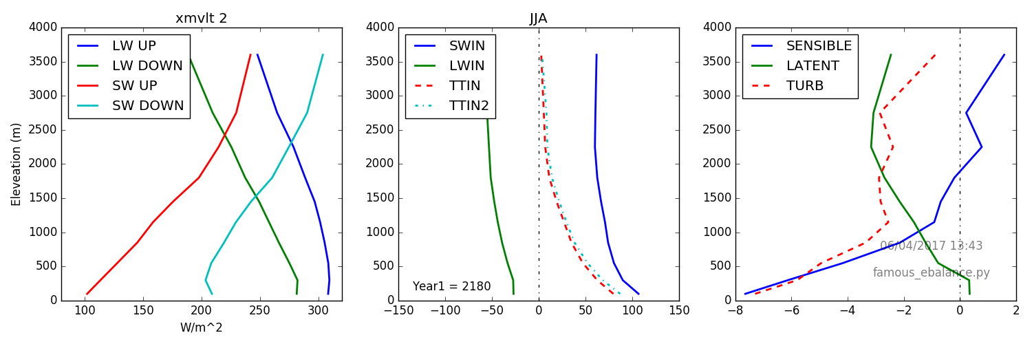
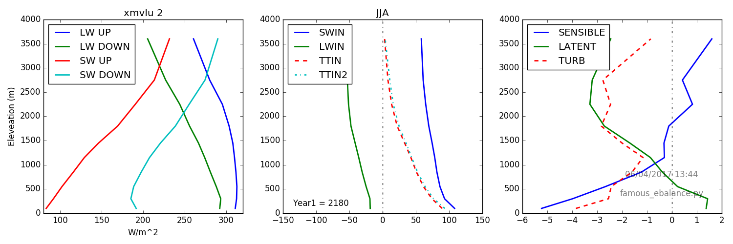
Tue Apr 18 16:56:36 BST 2017
There is also the question of the LW "lapse-rate". The energy balance plot for xmvlt above is repeated, but with the box (non-tiled) surface downward LW added. This is already a function wrt height, in the context of the normal UM radiation wrt (box average) elevation physics. The additional lapse-rate of the tiling scheme amplifies the existing LW decrease with height. Note: LWIN2 will be wrong, as I'm using the elevated-tile temperature to calculate LW out (just look at first plot). The differential lapse rate (i.e. of LWD - LWD2) is roughly -7.4 W m^2 per km. Figure 44(a): FAMOUS CTL (xmvlt) EB + LW2)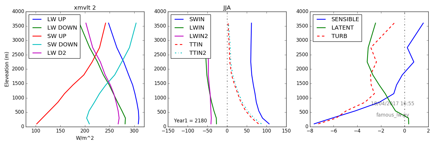
Wed Apr 19 18:03:43 BST 2017
Mapping the LW-down (LWD and LWD2) for each level: Figure 45: FAMOUS CTL (xmvlt) LW maps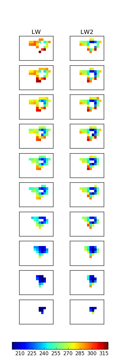
Thu Apr 20 14:34:23 BST 2017
Turbulent heat flux analysis (using literature formula). Positive flux is down. Figure 46: FAMOUS Turbulent Heat flux look-see (xmvlq)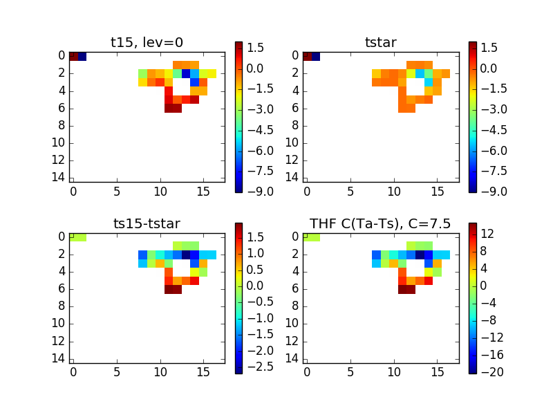
Mon Apr 24 13:08:22 BST 2017
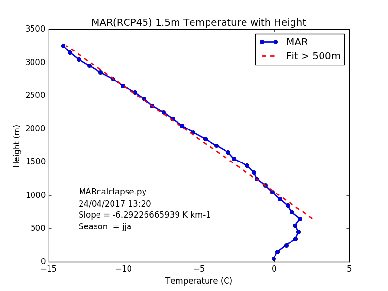
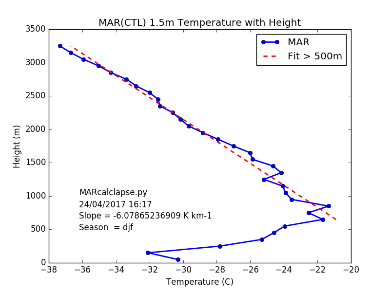
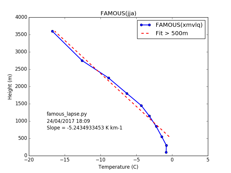
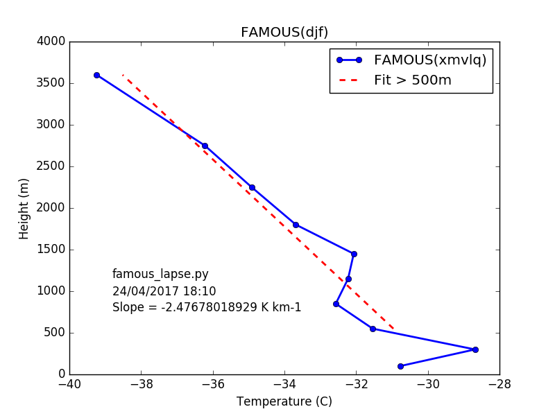
Calculate the effective atmosphere lapse rate over ice in the the MAR runs. The 1.5m temperatures are averaged over 100m altitude bands. Lower altitudes exhibit an inversion layer, with RCP45 exhibiting an obvious positive temperature (melt) region. Above ~500m bove models exhibit a lapse rate of ~-6.3 K km-1. The lapse rate is similar in winter (Fig. 47e), but with a more pronounced low-level inversion. Figure 47a: MAR(CTL) temp lapse rate (jja)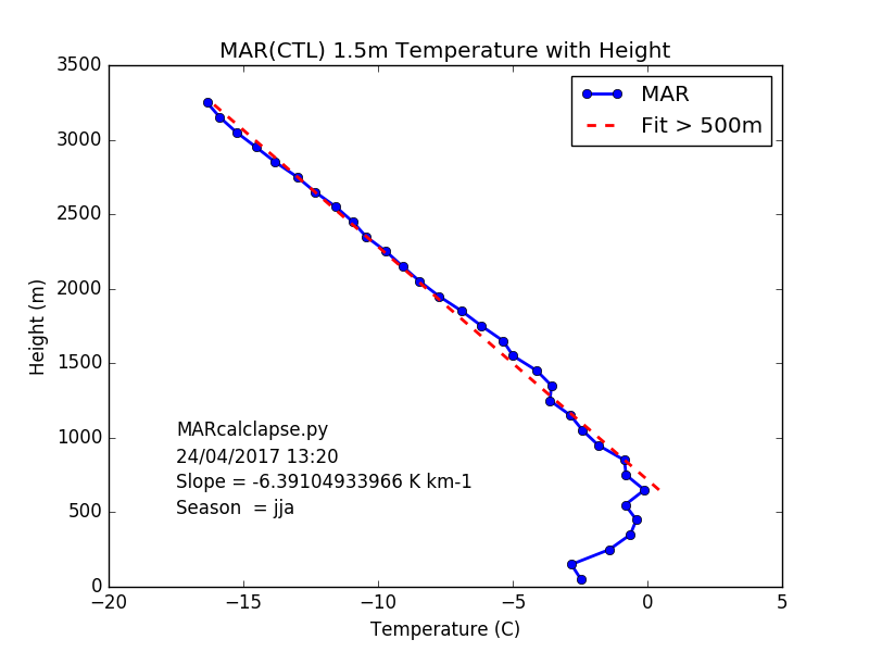
- xmvlt: from 2187.
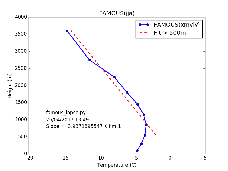
Tue Apr 25 10:24:40 BST 2017
Looking at the effective (over ice, area integral) lapse rate for the run (xmvlt) with a fixed tile adjustment temperature lapse rate. Figure 49a: FAMOUS(CTL:xmvlt) temp lapse rate (jja)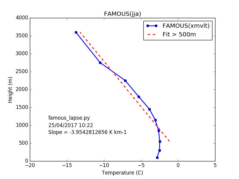
- xmvlv: Copy of xmvlt. From 2157 (30 years).
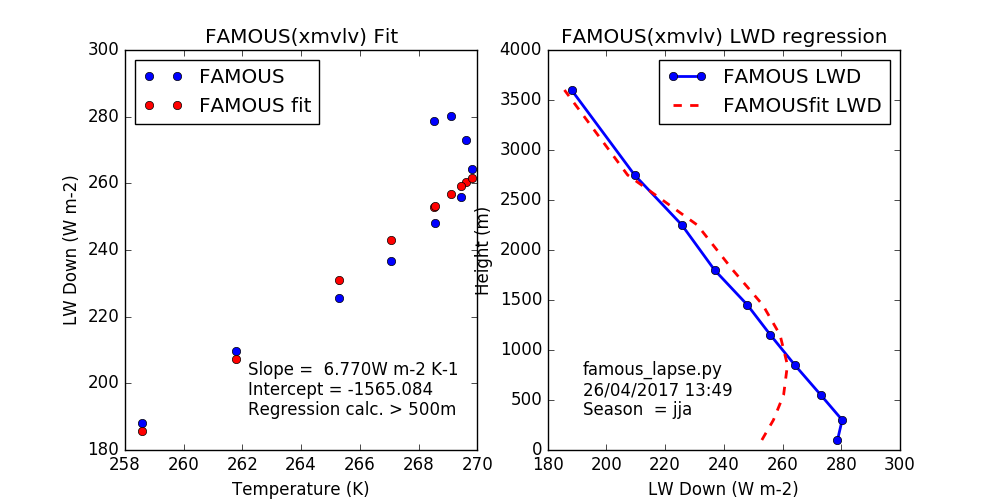
Wed Apr 26 10:51:22 BST 2017
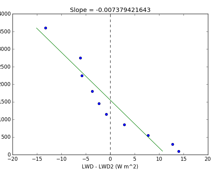
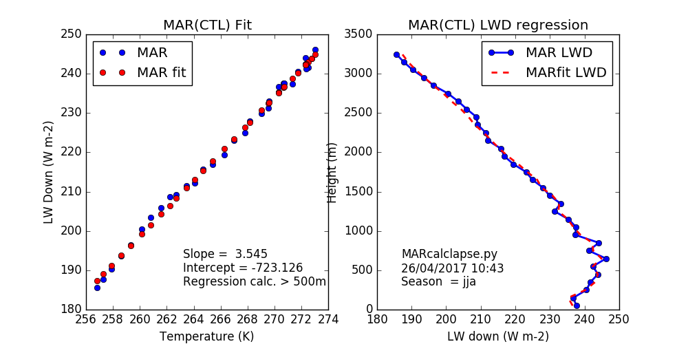
Note: Figure 47d corrected. Left hand plot has axes flipped (wrt labelling). Slope is 3.545 W m-2 K-1. Version of Figure 47d, but for FAMOUS (xmvlq). Slope is 5.333 W m-2 K-1. Figure 50a: FAMOUS(CTL:xmvlq) LWD regressed from temperature(jja)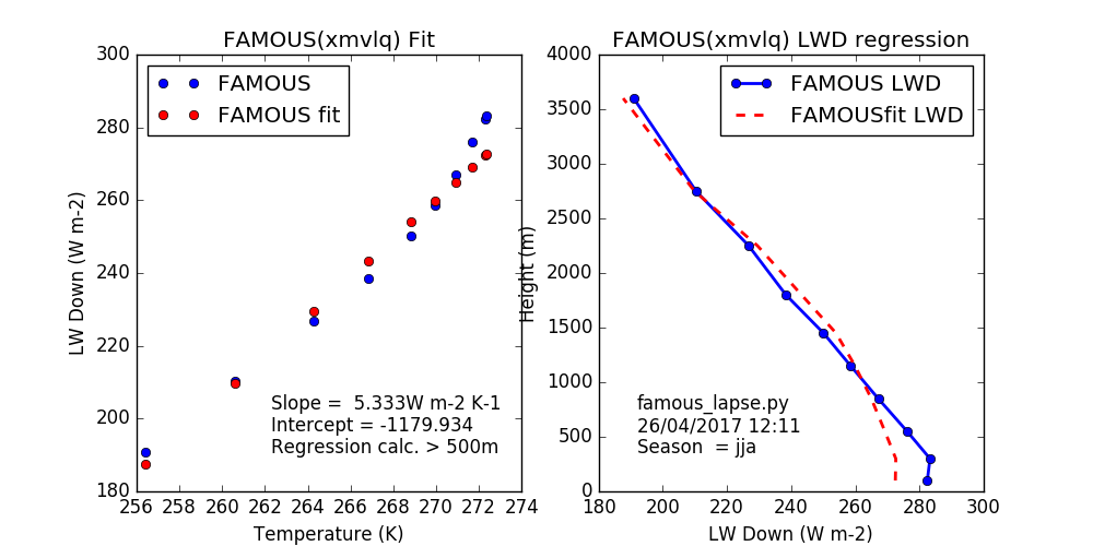
New run (xmvlv) with 6K km-1 lapse on tiles
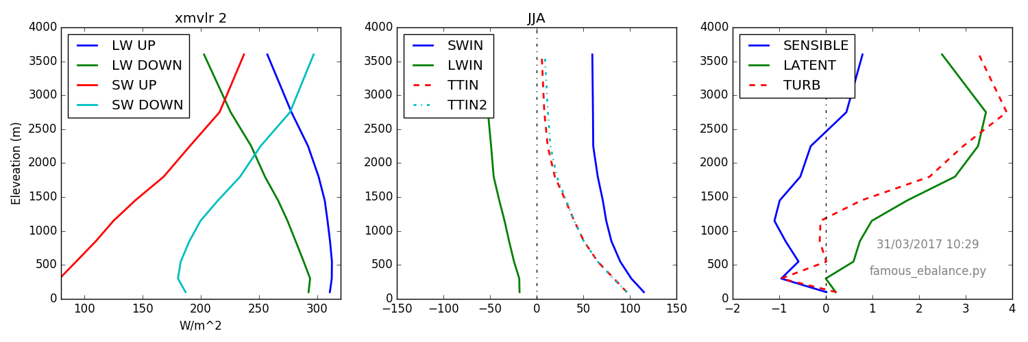
Figure 51a: FAMOUS(CTL:xmvlv) Integrated (area) Energy Balance (jja)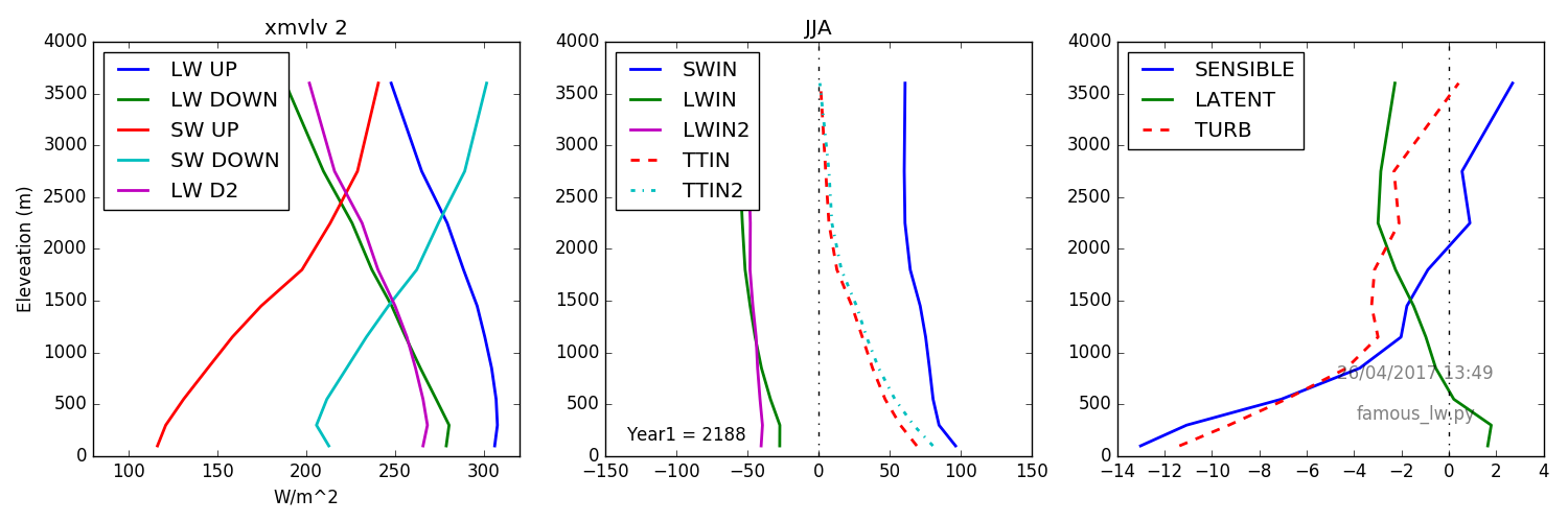
Fri May 19 12:01:18 BST 2017
NOTE: previous results from some runs are dubious due to sign of lapse rate being reversed. Runs compromised:- xmvlt: 3K/km tlapse (CTL)
- xmvlu: (RCP45)
- xmvlv: 6k/km tlapse (CTL) RERUN
- xmvlw: (RCP45) RERUN
- xmvlx: 6K/km tlapse;dLWdT = 5.4 (CTL) RERUN
- xmvly: (RCP45) RERUN
- xnkub: 6K/km tlapse;dLWdT = 3.6 (CTL)
Wed May 24 12:14:25 BST 2017
In bl_ic7a.f:
        tgrad=-0.006
! Specific humidity gradient still locally calculated
        qgrad=(q(i,BL_LEVELS)-q(i,1))/bldepth

        dLWdT  = 3.6
        lwgrad = dLWdT * tgrad
Figure 61a: FAMOUS(CTL:xnkub) SMB components
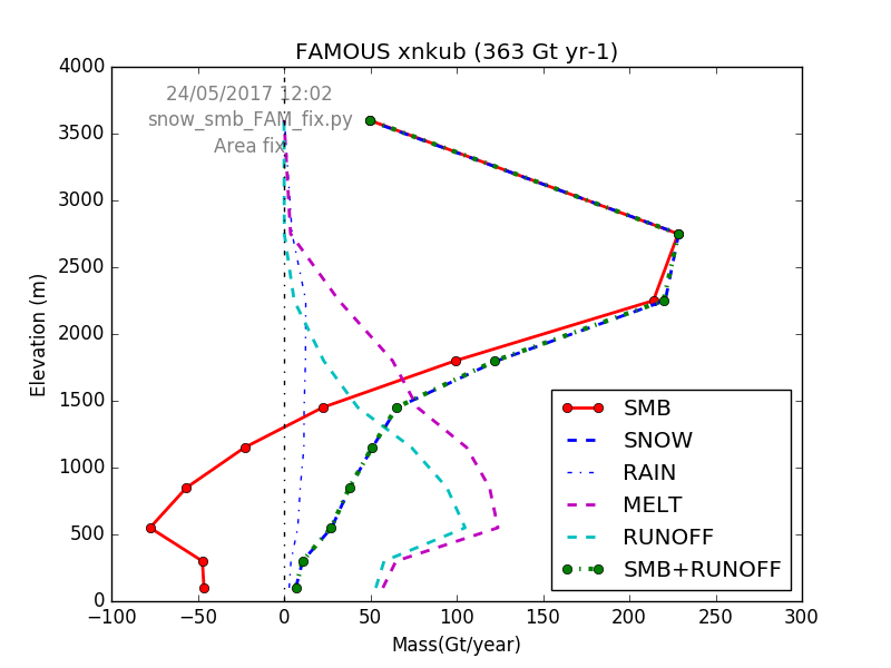
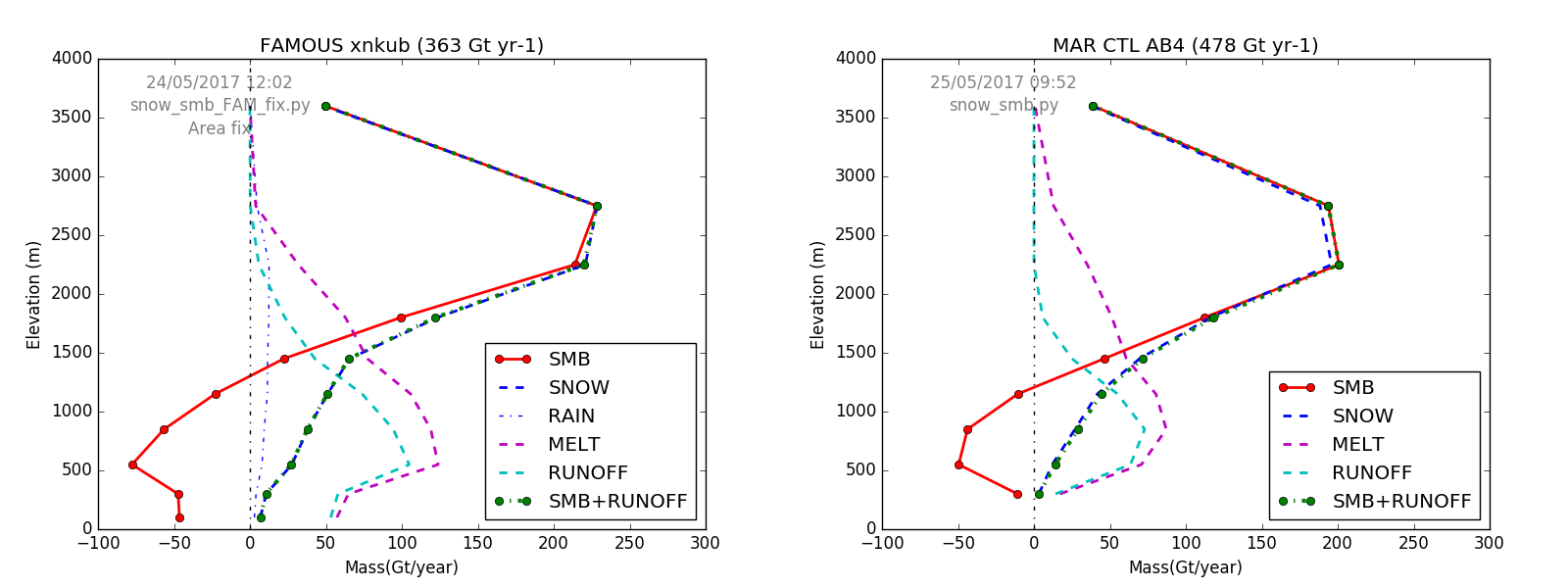
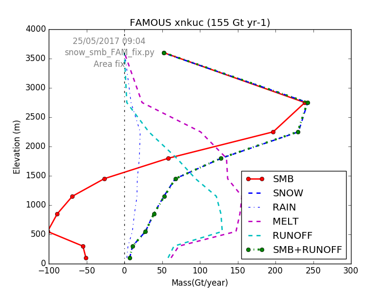
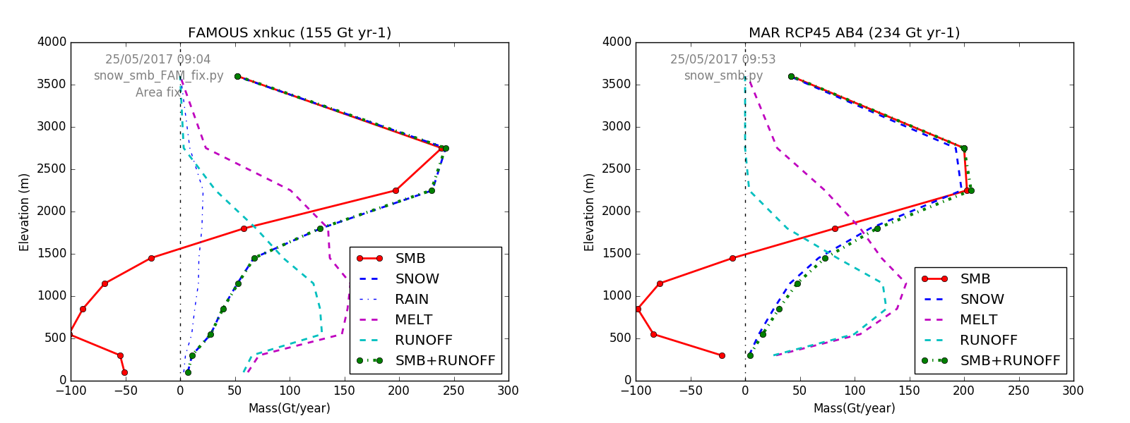
Change of SMB between CTL and RCP45
FAMOUS: 363-155 = 208 Gt/yr MAR: 478-234 = 244 Gt/yrThu Jun 29 10:05:23 BST 2017
New horizonal/vertical scheme implemented GCM→GLIMMER. Figure 62a: Ice sheet ACAB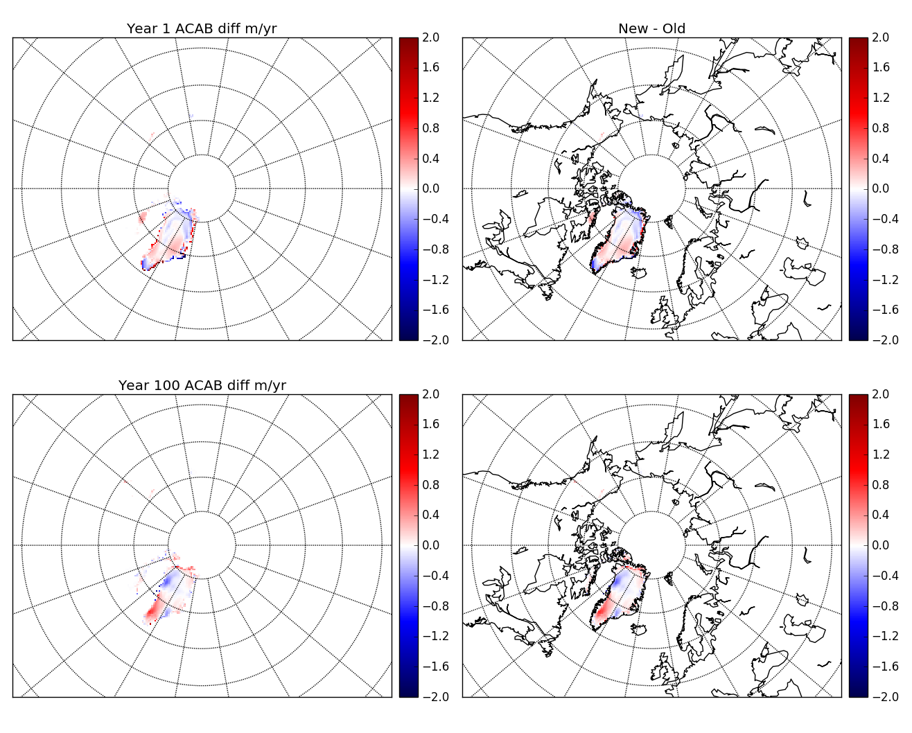
Fri Jun 30 11:57:53 BST 2017
Reference (coupled FAMOUSA/GLIMMER) experiments
Thu Jul 6 16:10:32 BST 2017
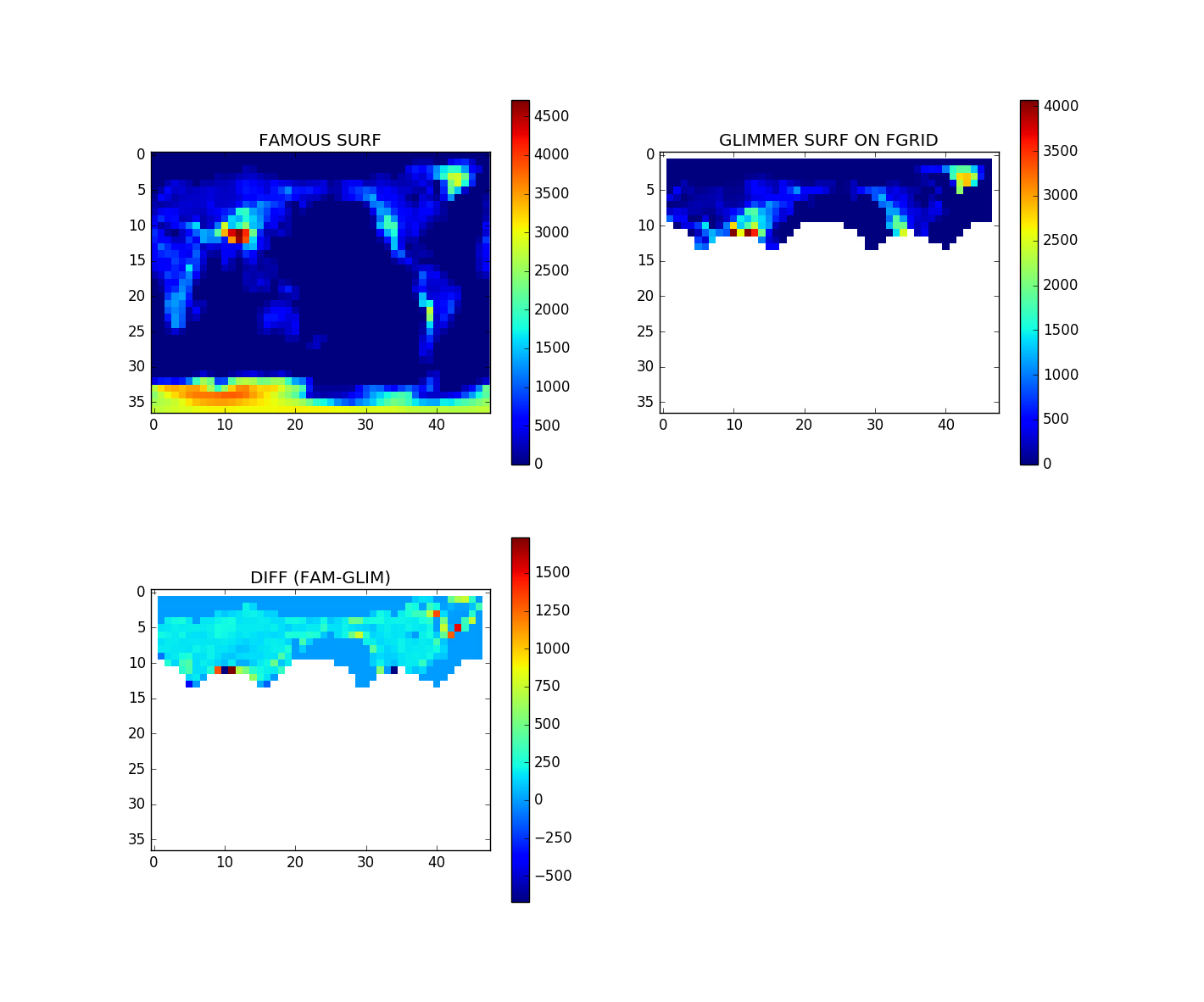
Topography issues; what is real?Looking at Figure 63a, with particular attention to the third row down. FAMOUS BG is the initial model orography (year 1), before coupling to the ice sheet. FAMOUS AG represents the orography after coupling. Third column is the difference field. The interactive region (i.e. vals > 0) is (on average) ~ 200m lower in the GLIMMER topography.
I did some offline calculations betwen the FAMOUS/GLIMMER data and this is confirmed in Figure 63b (a rough downscaling of the GLIMMER orography to that of FAMOUS gives similar results; so it's not a model issue).
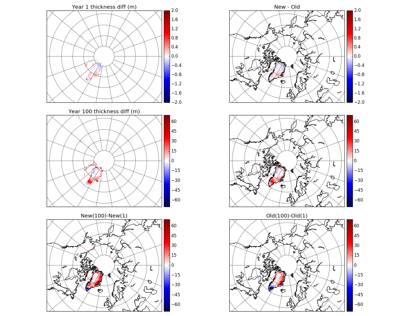
The final row in Fig 63a shows the difference on height between our FAMOUS and the portable version. Generally, the portable version has lower elevation, though the Himalayas are higher.
I'm looking for some advice on this. One issue is what happens at the boundaries between the GLIMMER sub-domain and the surrounding model space (mountain ranges introduced).
One option, is to make the sub-domain Greenland only and try and match the orography (and the elevation fractions etc).
Figure 63a: Topography comparision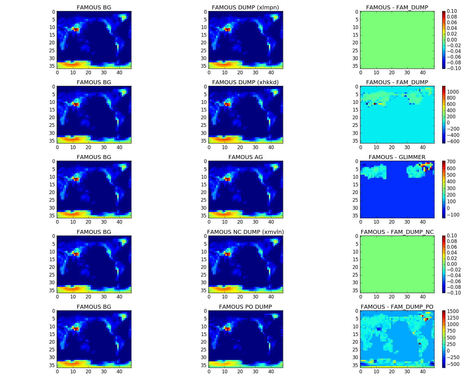
Fri Jul 7 00:28:50 BST 2017
Similar results comparing FAMOUS surface elevation with TBASE downscaled 2-minute data. Above zeros average difference ~200m. Figure 64a: Topography comparision (FAM vs TBASE)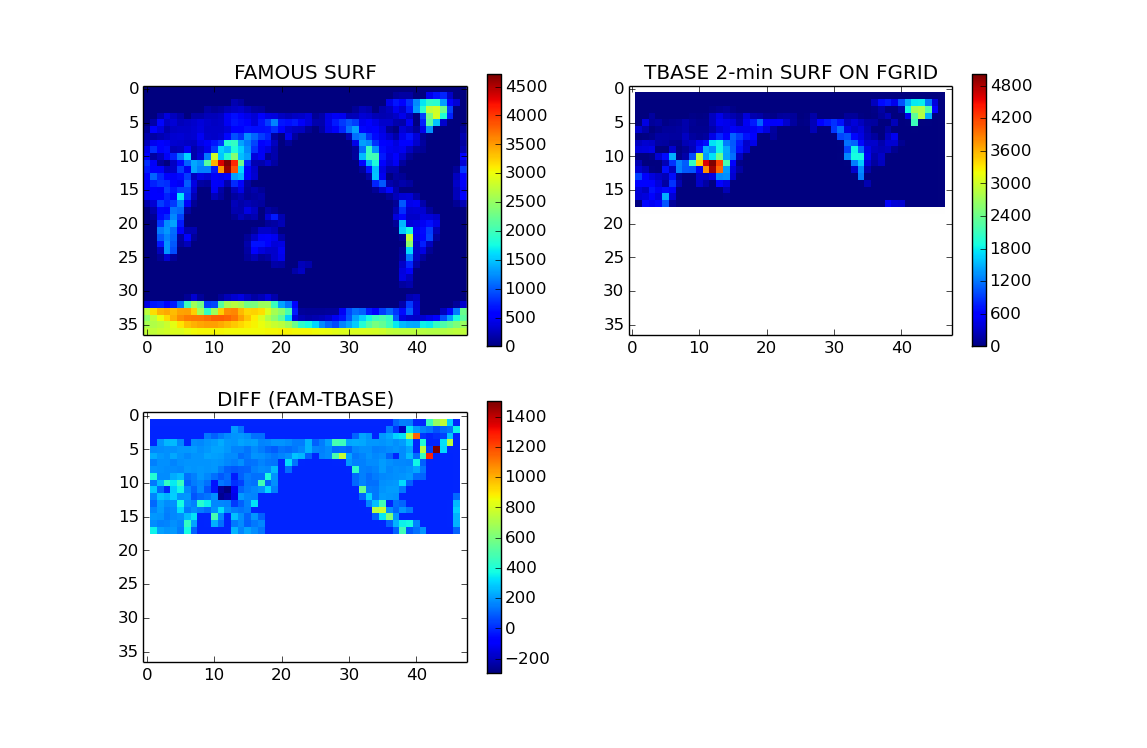
Tue Jul 11 20:00:28 BST 2017
New coupled setup (xnfuc). GLIMMER domain is now over Greenland only; as might be expected, the initial topographic adjustment is only over said region. Figure 65a: Topography comparision (GLIMMER domain now Greenland only)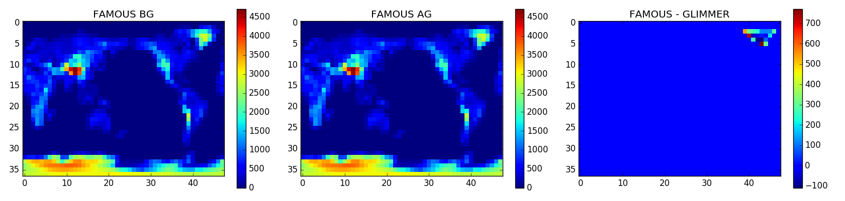
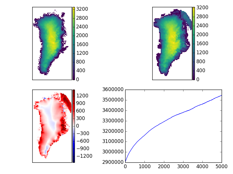
Thu Aug 10 10:08:09 BST 2017
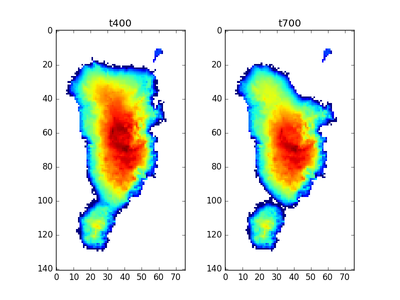
Offline spinup (5000 years, with xnkub SMB. Figure 66b is from a run that tries to do something clever with the non-ice snow field (and fails). Figure 66a: Ice sheet thickness: yr1, yr5000 and diff. Plus ice volume (km3)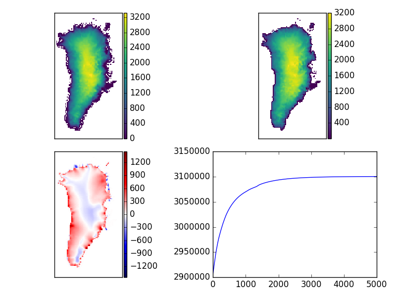
Mon Aug 14 14:28:07 BST 2017
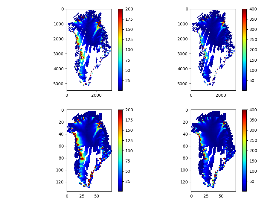
Modelled and observed surface ice velocities; modelled values are from offline pinup (i.e., ice-model with non-evolving SMB). Figure 67a: Ice surface velocity (magnitude) m/yr (model)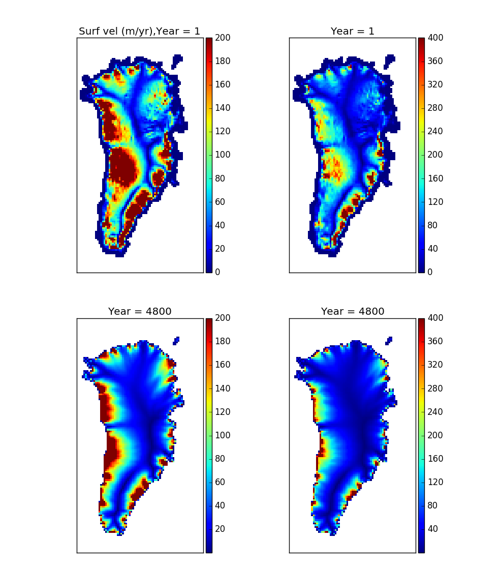
Tue Aug 15 11:12:31 BST 2017
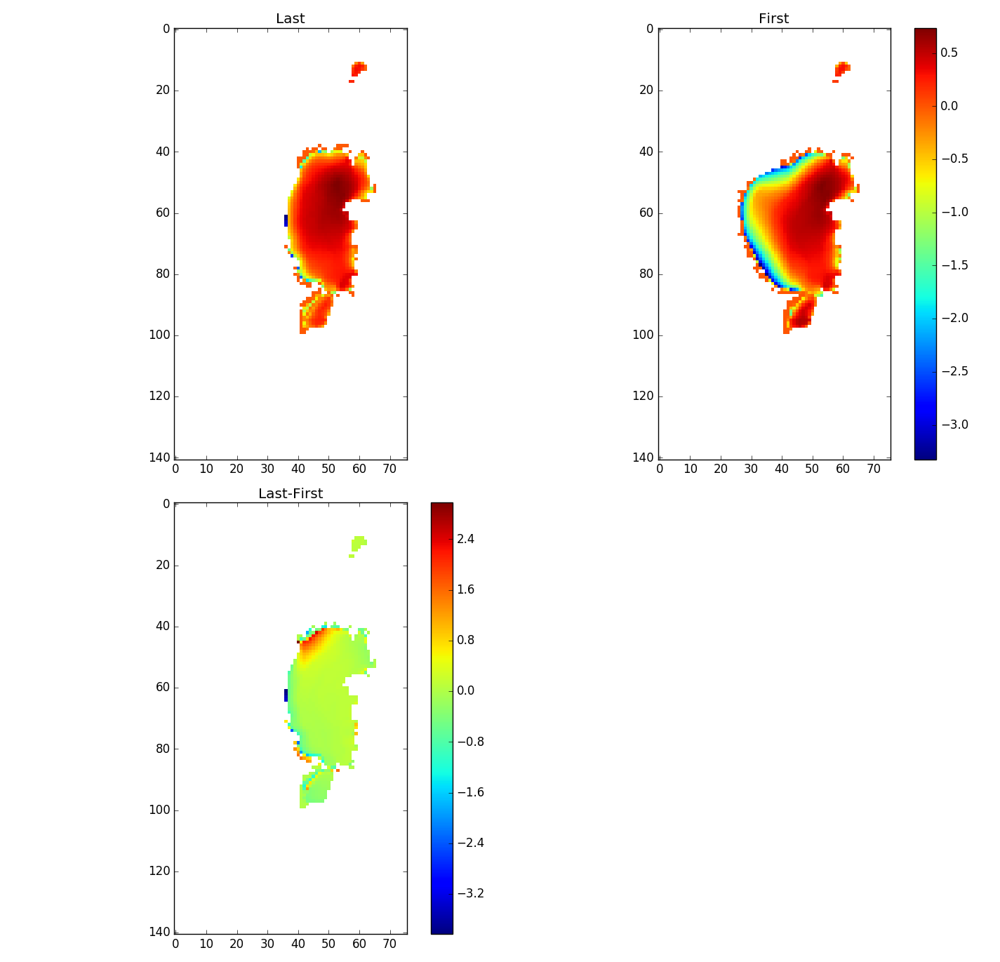
Interestingly, if you define the ice-shit run as using a 'hotstart' it expects to find a 3D temperature field in the input file ... but doesn't complain if it's not there (just creates a random, non-physical temp field). Figure 68a: Ice temperature (model)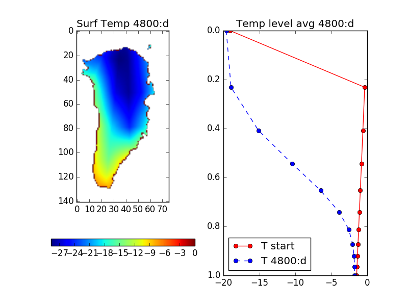
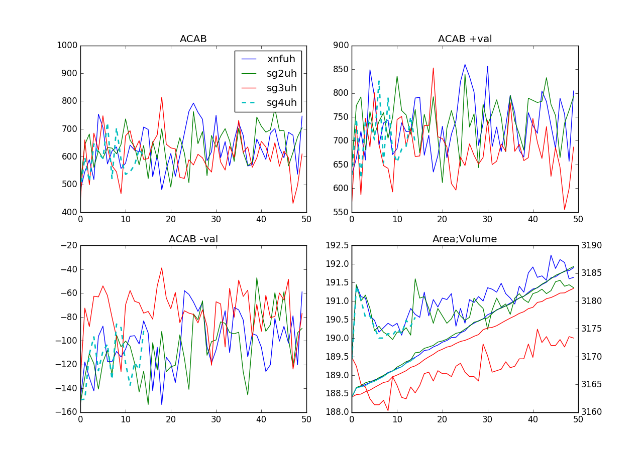
Fri Sep 8 10:30:58 BST 2017
- xnfuh: 3D Interpolation masks, with average SMB per elevation.
- sg2uh: 3D Interpolation masks, with halo SMB
- sg3uh: No 3D interpolation mask
- sg4uh: As xnfuh but with average elevation SMB set to zero.
Fri Oct 6 14:21:31 BST 2017
Job monitorTue Nov 7 14:56:15 GMT 2017
Updated: Thu Nov 9 11:11:12 GMT 2017 Figure 70: Volume difference with nasty snow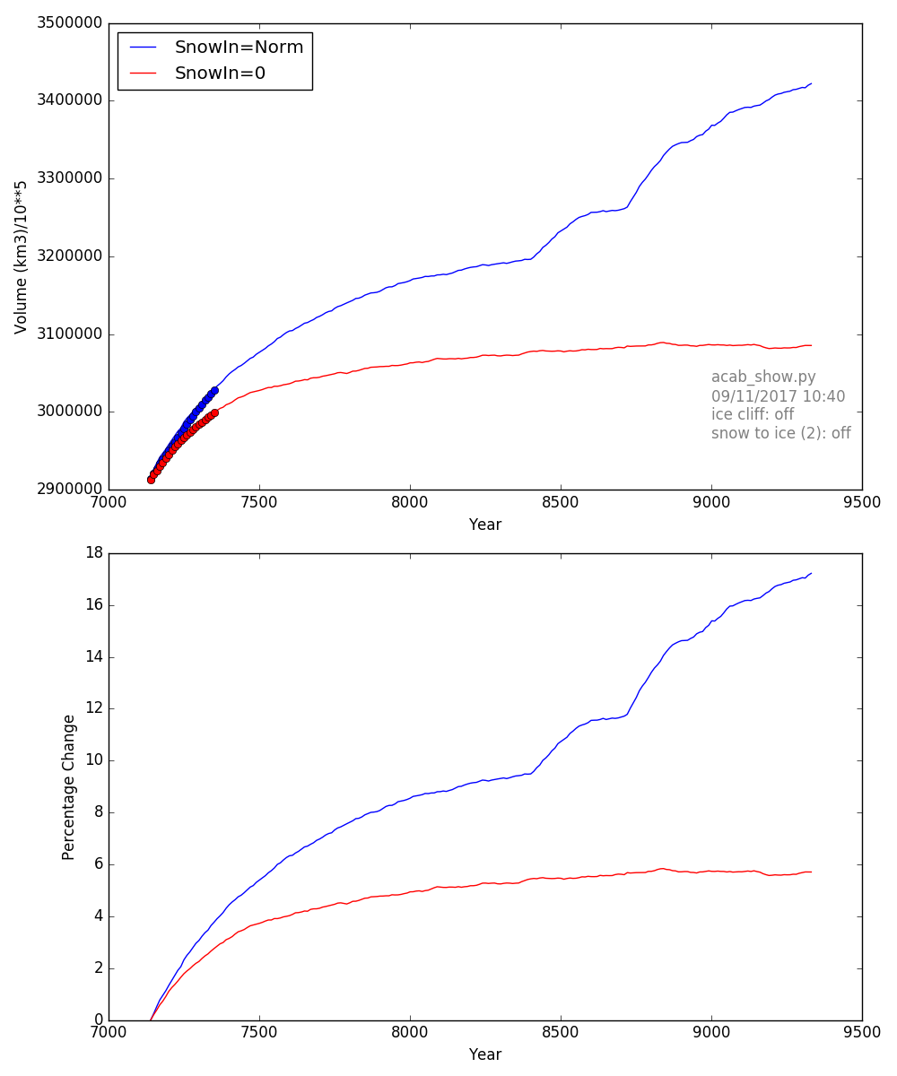
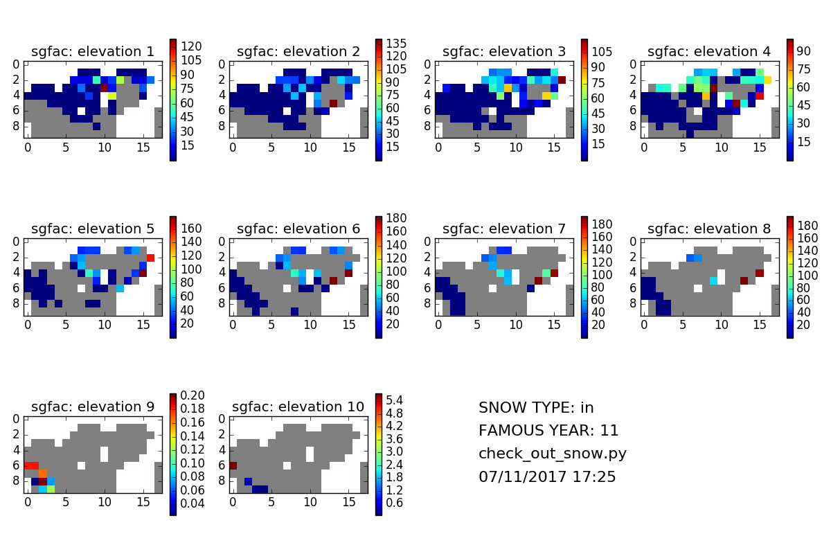
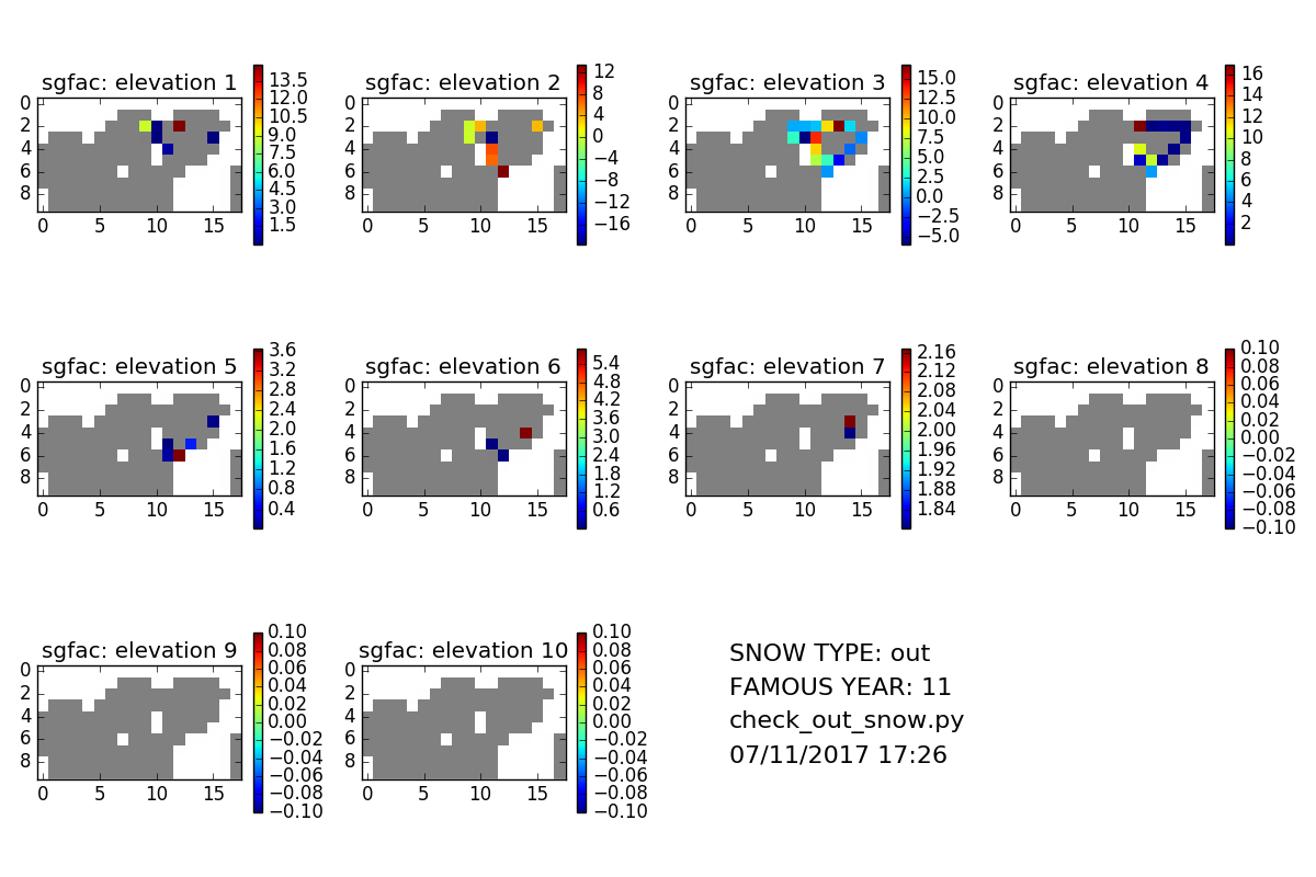
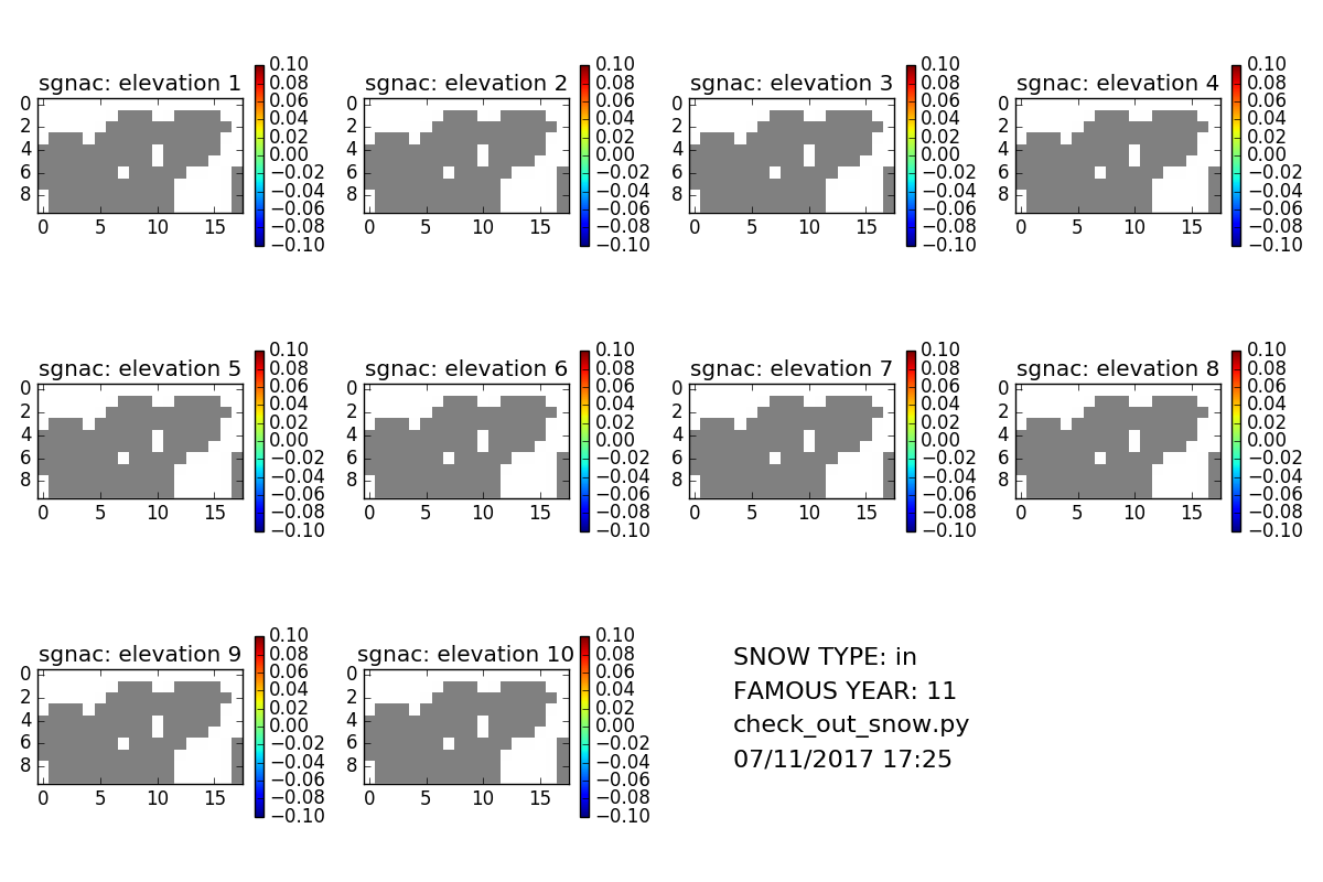
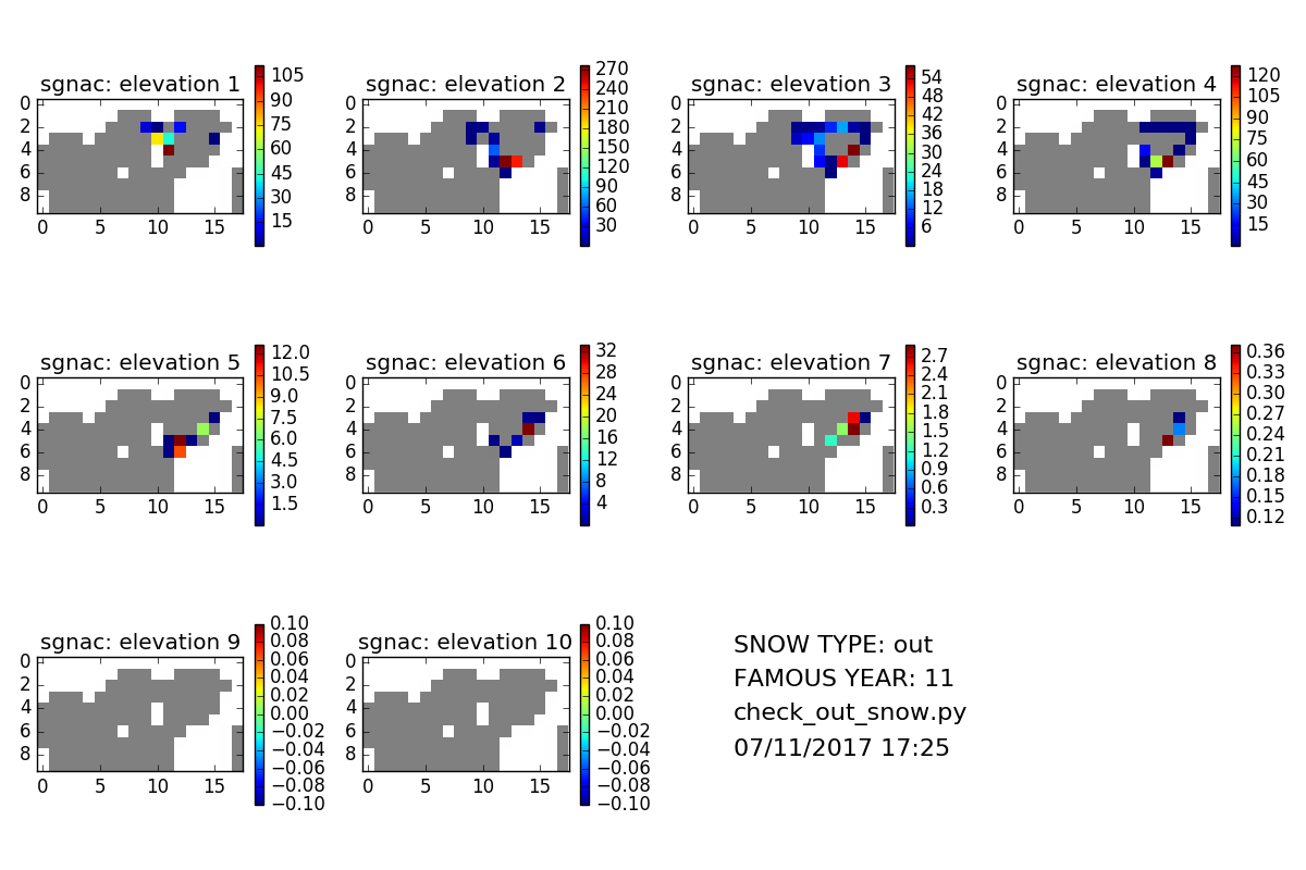
Non-ice snow in out of GLIMMER (on FAMOUS side)
- sgfac: Snow in as per normal (x10 accel).
- sgnac: Zero (non-ice) now in (x10 accel).
Wed Nov 8 17:13:44 GMT 2017
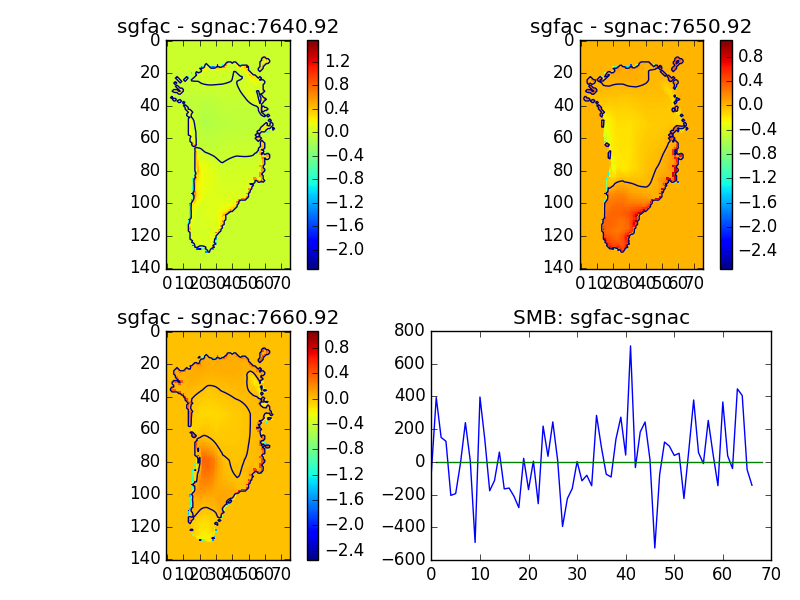
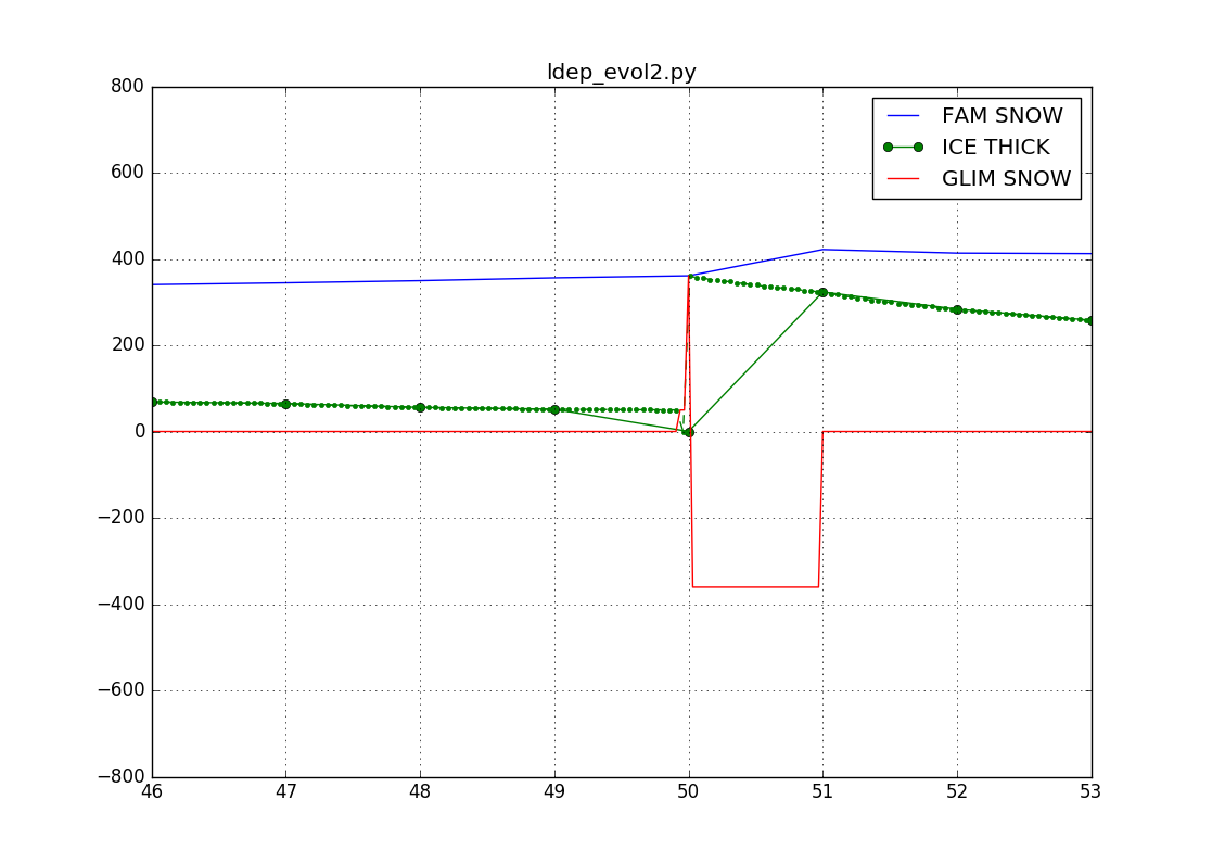
Contemplating. Ice erodes but snow accumlates. Switches to ice when ice is zero. And so the process repeats. Anomalous accumulation point (in FAMOUS) ... biasing the GLIMMER input as smoothed over a large area. Figure 73: Ice to no ice to ice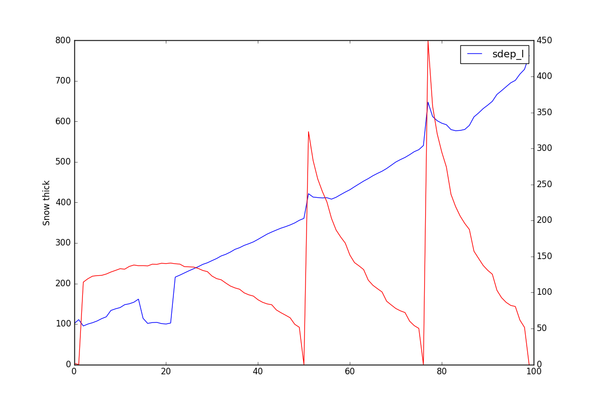
Thu Nov 9 10:28:26 GMT 2017
Figure 74: Non-ice snow smearing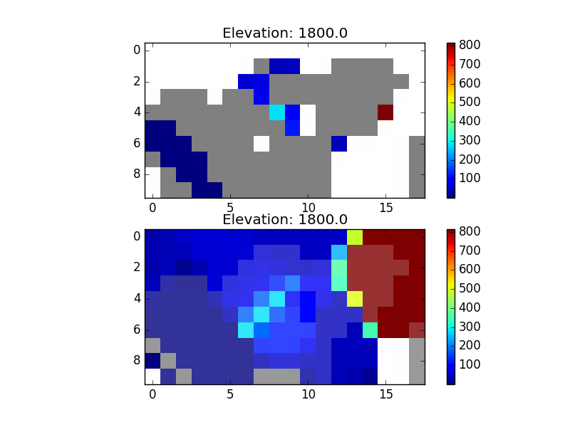
Figure 75: Ice breakout from mask
Mon Nov 20 13:07:23 GMT 2017
Mass accumulation issues.Thu Nov 23 17:57:04 GMT 2017
A closeup of plot 73.Description
- Blue line is "potential" non-ice snow; interp from FAMOUS to GLIMMER space.
- Green line is ice-thickness in FAMOUS timesteps; dotted lines are internal accel steps.
- Red line is actual non-ice snow developed in GLIMMER space (accel time steps)
Process
- Ice is being ablated, and near the end of tstep49 ice is turned to snow.
- This amount of snow should be sent back to FAMOUS, and be part of the blue line at tstep50
- At tstep50 the box is free of ice, potential snow is turned into actual snow; red jump to blue.
- This is turned into ice and the snow converted into a negative anomaly to send back to FAMOUS.
- At tstep51 one would expect potential snow to be reduced, but it has increased.
- This is why I thought there was a sign error somewhere (but could find nothing).
Mon Dec 4 18:02:22 GMT 2017
New CTL run with outmask turned off. Also, outside the mask, the bathymetry is now set to -3000m. RCP85 run started from a seemingly settled GrIS volume. Figure 77: Ice sheet evolution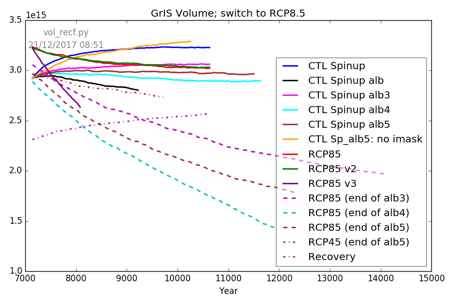
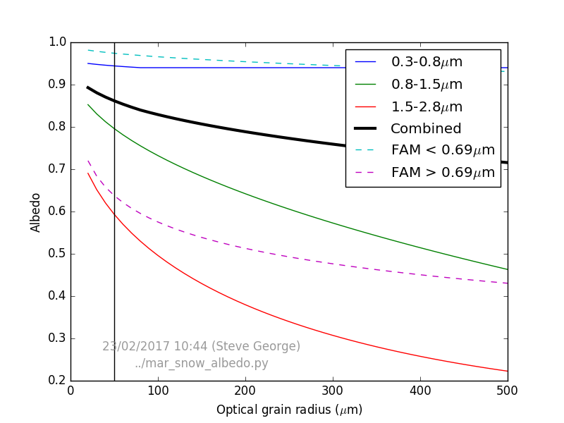
Snow Albedo
Considering the snow albedo, I've started another control run with a more realistic (visible) snow albedo (Roesch[2002]). Offline calculation of albedo ranges below. After ∼500 years, GrIS is only experiencing a modest increase in volume (see above). Figure 78: Snow albedo with grain size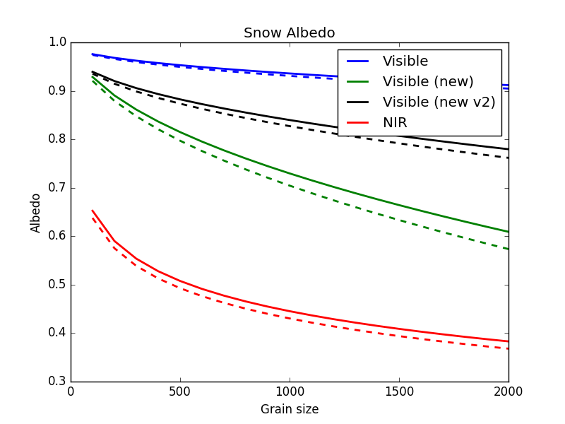
Tue Dec 5 15:40:17 GMT 2017
Seasonal evolution of grain size on ice and non-ice tile fractions (one year). It's a bit messy, but the takehome is that we're only getting chunky grains on the ice fractions (which sounds correct). On the lowest elevation, non-ice snow grain size gets up to ∼1600 microns ( ∼0.65 albedo). Figure 79: Snow albedo height/month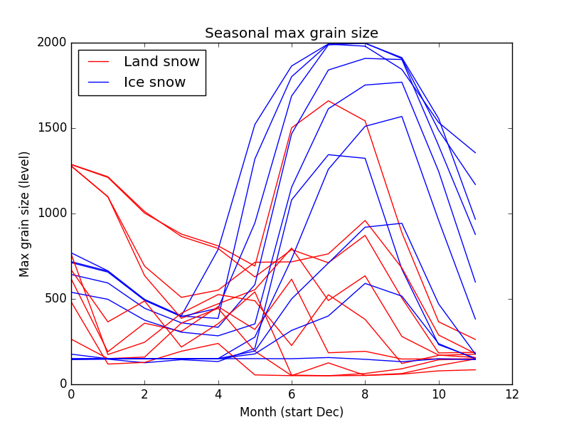
Thu Dec 14 10:43:29 GMT 2017
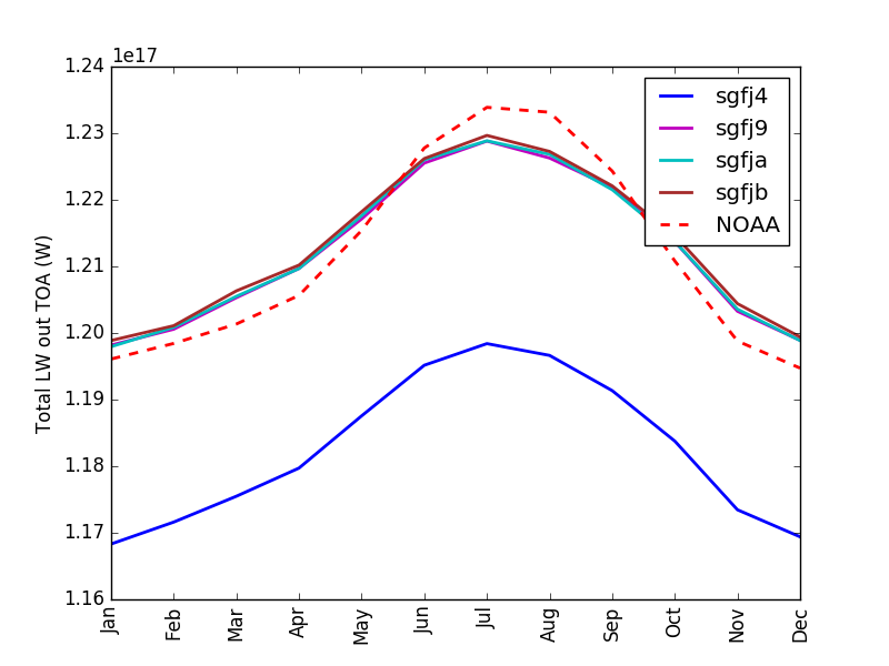
Looking at OLR TOA. The coupled FAMOUS/ice model with the original high albedo in the visible spectrum has a reduced OLR TOA. I assume this reflects the increased SW reflected by the big, shiny high ice blob.| Source | Annual average W/m^2 |
|---|---|
| Standard FAMOUS ref xfhcu | 237.322 |
| Back of envelope | 239.00 |
| NOAA 1degree | 237.541 |
| FAM_ice original albedo sgfj4 | 231.831 |
| FAM_ice albedo3 sgfj9 | 237.685 |
| FAM_ice albedo4 sgfja | 237.714 |
| FAM_ice albedo5 sgfjv | 237.835 |
As per Figure 61
Figure 81: SMB components (cyan CTL)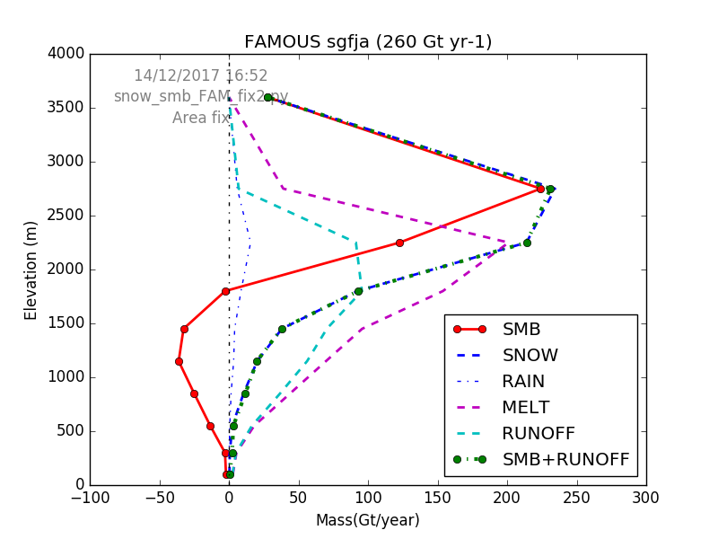
Fri Dec 15 11:56:40 GMT 2017
As per Figure 61
Figure 82a: SMB components (magenta CTL: sgfj9)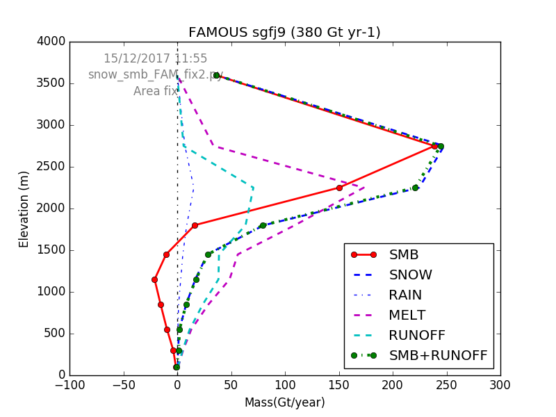
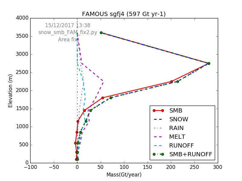
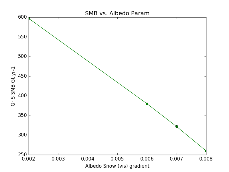
Figure 83: SMB vs. Albedo parameter)
Mon Dec 18 13:02:58 GMT 2017
Figure 84: Anim 1
Wed Dec 20 10:14:42 GMT 2017
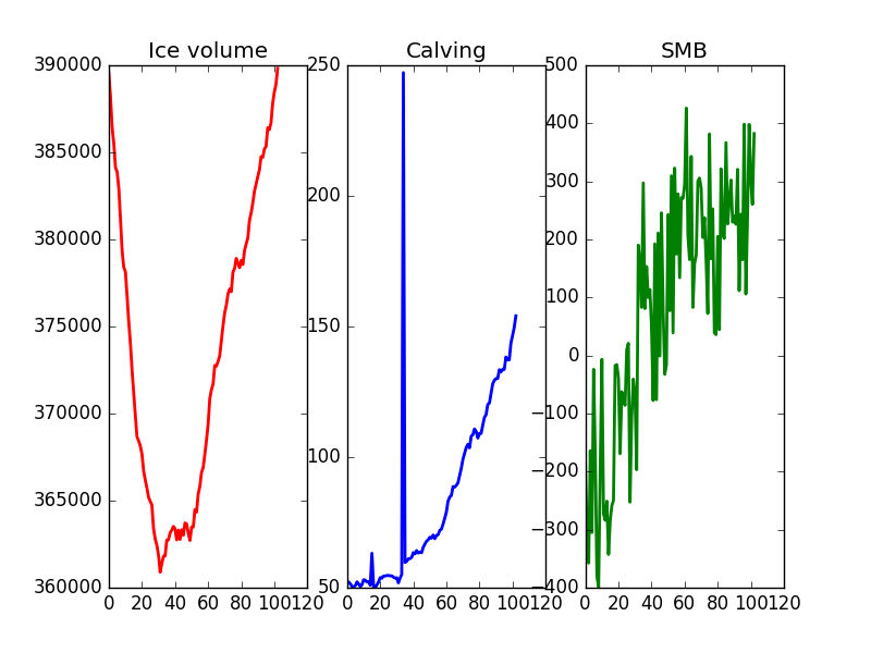
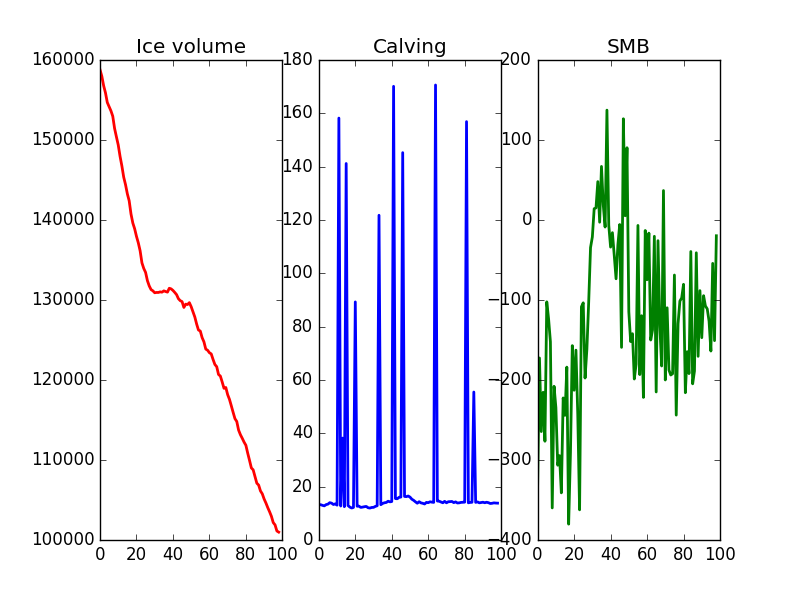
Started a new CTL run (brown variant), with non-constrained ice. So far, there is some spread (as to be expected without a significant percent of required calving), but it's not looking too bad. The new run is in orange in the general development plot, and here is a map of the ice-thickness evolution (so far). Figure 85: ice thickness, no constraint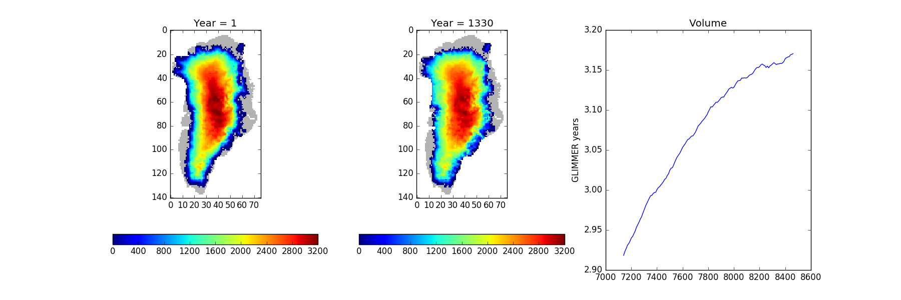
Tue Feb 13 11:27:33 GMT 2018
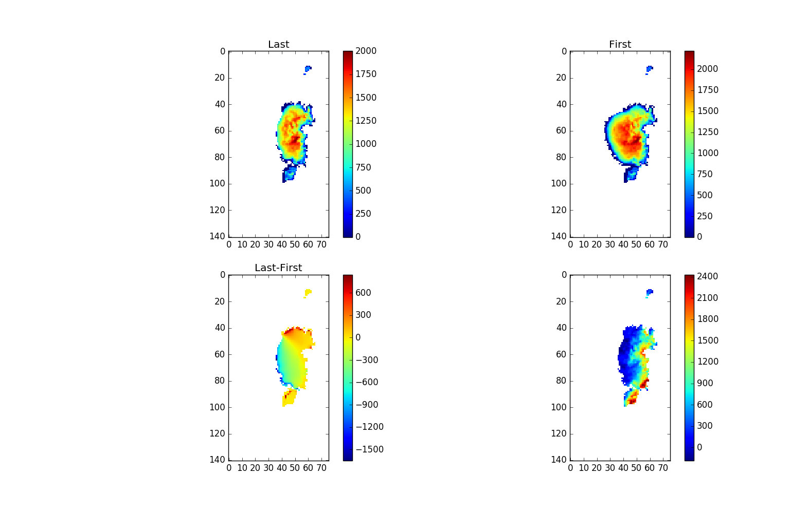
Looking at the endstates for some of the longer rcp85/4xCO2 runs. Figure 86: Ice sheet endstates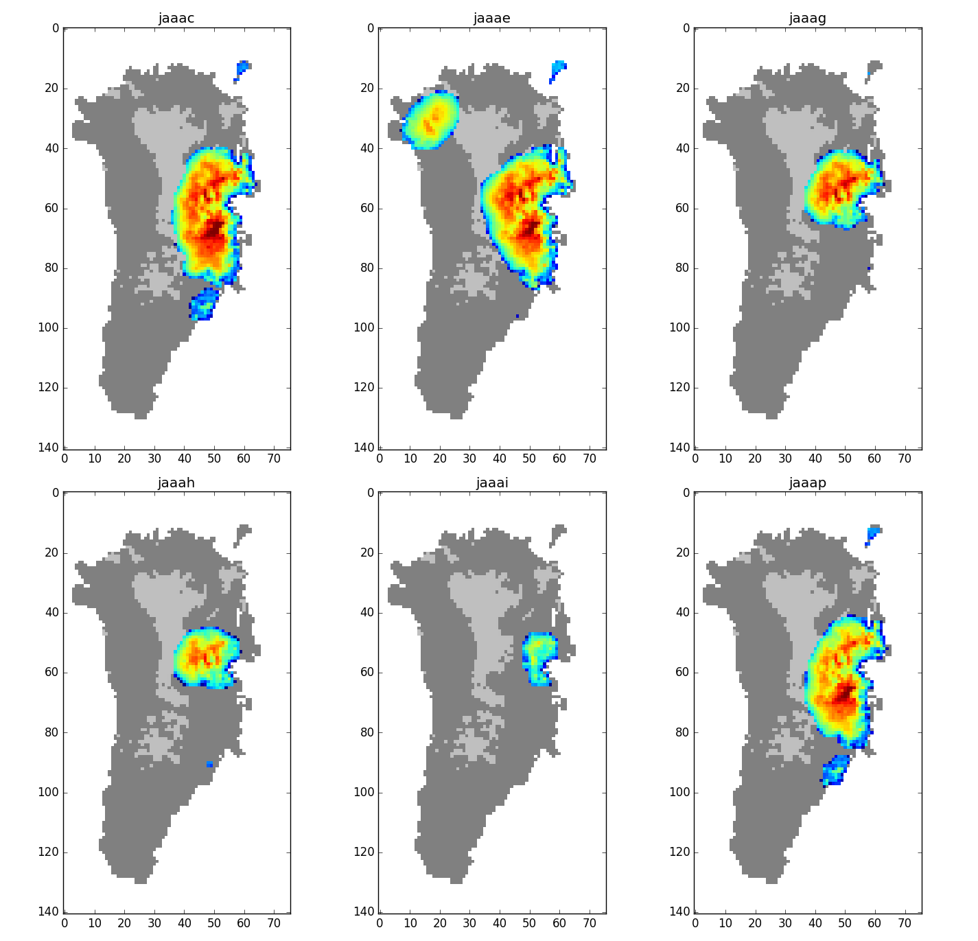