ESM2025 Notebook
Fri 6 Jan 12:56:49 GMT 202
Farfield forcing calculation from NEMO data
Thermal forcing (TF) is the difference between in the in situ temperature and the local freexing point of water.
NEMO output is on a tripolar grid. The following scripts regrid to a 1-degree standard lat/lon grid, which is then further projected onto the Bedmap stereographic (equidistant) grid. Average TF are calculated for each of the 7 regional polygons defined by the ISMIP6 documentation.
Script: Reformat NEMO data into standard 1-degree grid
import numpy as np
import pylab as py
import scipy
import math
import cf


# freezing point parameters
l1 = -5.73e-2
l2 = 8.32e-2
l3 = -7.53e-4


inf='out1.nc'

npt='thetao'
nsa='so'
ndp='deptht'   # Maybe use bounds


#inc=NetCDFFile(inf)

f=cf.read(inf)
ptemp=f.select('sea_water_potential_temperature')[0]
salin=f.select('sea_water_salinity')[0]

# subspace 200-500m depth in ocean
ptemps=ptemp.subspace(depth=cf.ge(200) & cf.le(500))
salins=salin.subspace(depth=cf.ge(200) & cf.le(500))

# Forcing
sdepth=ptemps.coordinate('depth').array
l3array=salins.data.array[0]
for i in range(len(sdepth)):
    l3array[i,:,:]=sdepth[i]*l3

#tforcs=ptemps - (l1*salins + l2 + l3*sdepth)
dblob=ptemps.data.array-(l1*salins.data.array + l2 + l3array)
TFs=ptemps.copy() # Thermal forcing
ix=np.where(salins.data.array < 0.001)[:]
dblob[ix]=np.nan
dblob=np.ma.masked_invalid(dblob)
TFs.data=dblob

TF=TFs.collapse('depth: mean',weights=True)
rg=False
rg=True

if rg:
 lat1=py.arange(-89.5,90.5,1)
 lon1=py.arange(0.5,360.5,1)
 nx=lon1.size
 ny=lat1.size
 properties = {'standard_name': 'potential temperature'}
 dimY = cf.DimensionCoordinate(data=cf.Data(lat1))
 dimY.set_properties({'standard_name': 'latitude','units': 'degrees_north'})
 dimX = cf.DimensionCoordinate(data=cf.Data(lon1))
 dimX.set_properties({'standard_name': 'longitude',
                      'units': 'degrees_east'})
 bounds_array = np.empty((ny, 2))
 bounds_array[:, 0] = lat1 - 0.5
 bounds_array[:, 1] = lat1 + 0.5
 bounds = cf.Bounds(data=cf.Data(bounds_array))
 dimY.set_bounds(bounds)
 bounds_array = np.empty((nx, 2))
 bounds_array[:, 0] = lon1 - 0.5
 bounds_array[:, 1] = lon1 + 0.5
 bounds = cf.Bounds(data=cf.Data(bounds_array))
 dimX.set_bounds(bounds)


 g=cf.Field(properties=properties)
 domain_axisY = cf.DomainAxis(ny)
 domain_axisX = cf.DomainAxis(nx)
 axisY = g.set_construct(domain_axisY)
 axisX = g.set_construct(domain_axisX)

 data = cf.Data(np.zeros([ny,nx]), 'K')
 g.set_data(data)
 g.set_construct(dimY)
 g.set_construct(dimX)

#
 r_TF=TF.regrids(g, method='bilinear', src_axes={'X': 'ncdim%x', 'Y': 'ncdim%y'}, src_cyclic=True)
 r_TF.del_construct('measure:area') # Bug fix. Cell areas should't be there

 # 2D thermal forcing on regular grid
 cf.write(r_TF,'TF2.nc')
import numpy as np
import pylab as py
import scipy
import math
import cf
from pyproj import Proj
import scipy.interpolate as interp
import scipy.io as sio
from shapely.geometry import Point, Polygon

def getoceanreg():
  indir='/home/tp909989/Projects/ESM2025/ISMIP6/ISMIP6/ismip6-gris-ocean-processing-master/final_region_def/'
  infile=indir+'ice_ocean_sectors.mat'
  test = sio.loadmat(infile)

  regdict={
          "regions": "ocean",
          "number" : 7,
          }
  regions=test['regions']
  for k in range(7):
    x=np.squeeze(regions[0,k][1][0][0][0])  # ocean x
    y=np.squeeze(regions[0,k][1][0][0][1])  # ocean y
    xlen=len(x)
    llist=[]
    for j in range(xlen):
       llist.append((x[j],y[j]))
    #dum=np.array([x,y])
    poly=Polygon(llist)
    regdict[str(k+1)]= poly

  return regdict

py.ion()
inf2='TF2.nc'
f2=cf.read(inf2)
TFin=f2[0]

latitude=TFin.construct('latitude').data.array
longitude=TFin.construct('longitude').data.array
ny=latitude.size
nx=longitude.size
lat,lon=np.meshgrid(latitude,longitude)
nbig=nx*ny
#lat_bnd=latitude-0.5
#lat_bnd=np.append(lat_bnd,latitude[ny-1]+0.5)
#lon_bnd=longitude-0.5
#lon_bnd=np.append(lon_bnd,longitude[nx-1]+0.5)


# Projection from NSIDC
myProj=Proj('+proj=stere +lat_0=90 +lat_ts=70 +lon_0=-45 +k=1 +x_0=0 +y_0=0 +datum=WGS84 +units=m +no_defs')
xx3,yy3=myProj(lon,lat)


dd = 50 # grid resolution in km
ddm = 50* 1000 #
xreg=np.arange(-3e6,3e6+ddm,ddm);nxreg=xreg.size
yreg=np.arange(-4e6,0e6+ddm,ddm);nyreg=yreg.size

indata=np.squeeze(TFin.data.array)
indataR=indata.reshape(nx*ny)[~indata.mask.reshape(nx*ny)]


inmask=indata.data.copy()
inmask[:]=1.0
inmask[indata.mask]=0
inmaskd=inmask.reshape(nx*ny)
xx2R=xx3.T.reshape(nx*ny)[~indata.mask.reshape(nx*ny)]
yy2R=yy3.T.reshape(nx*ny)[~indata.mask.reshape(nx*ny)]

points=np.array([xx2R,yy2R]).T
xx3m=xx3.T.reshape(nx*ny)
yy3m=yy3.T.reshape(nx*ny)
points2=np.array([xx3m,yy3m]).T


interpolator = interp.CloughTocher2DInterpolator(points,indataR)
intmask=interp.LinearNDInterpolator(points2,inmaskd)

outdata=np.empty([nyreg,nxreg])
outmask=np.empty([nyreg,nxreg])
# Interpolate data and mask
for ix in range(nxreg):
    for iy in range(nyreg):
        outdata[iy,ix]=interpolator(xreg[ix],yreg[iy])
        outmask[iy,ix]=intmask(xreg[ix],yreg[iy])


dum=py.where(outmask < 0.1)
outmask[:]=1
outmask[dum]=py.nan
outmask=np.ma.masked_invalid(outmask)
outdata=np.ma.array(outdata,mask=outmask.mask)

regions=getoceanreg()

xgrid,ygrid = np.meshgrid(xreg, yreg)

dum=outdata.copy()

TFsec=   {
          "regions": "ocean",
          "number" : 7,
          }

py.figure(4);py.clf()
for kk in range(7):
  dum[:]=py.nan
  davg=0;davgc=0
  davg2=0;davgc2=0
  for ii in range(nxreg):
    for jj in range(nyreg):
        pnt=Point(xgrid[jj,ii],ygrid[jj,ii])
        if pnt.within(regions[str(kk+1)]):
            dum[jj,ii]=1
            if ~outdata.mask[jj,ii]:
                davg=davg+outdata[jj,ii]
                davgc+=1
            davg2=davg2+outdata[jj,ii]
            davgc2+=1
  tavg=davg/davgc
  TFsec[str(kk+1)]=tavg
  py.figure(4)
  py.subplot(3,3,kk+1)

  py.imshow(py.flipud(outdata))
  py.imshow(py.flipud(dum),interpolation='none',cmap=py.get_cmap('rainbow'),vmin=0,vmax=1,alpha=0.3)
  py.title("Sector "+str(kk+1))
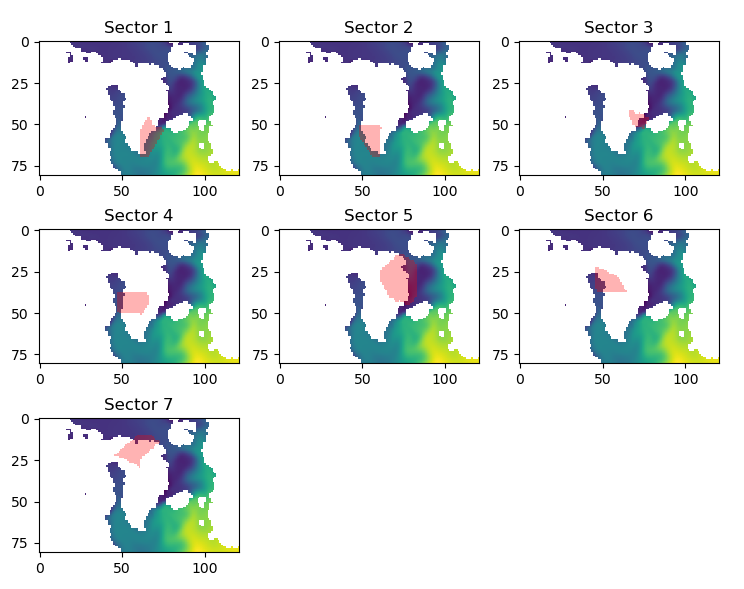
TF Forcing (C)
  Sector 1 = 6.388450930530248
  Sector 2 = 6.121850990176432
  Sector 3 = 2.273225817670175
  Sector 4 = 3.7989264943999914
  Sector 5 = 2.2589612622503217
  Sector 6 = 3.0936962158457333
  Sector 7 = 2.7306765218024744
Fri 13 Jan 13:07:41 GMT 2023
Variability of TF with time. Data from CMIP6 piControl (UKESM).Figure: Change of TF with time
Mon 23 Jan 22:31:26 GMT 2023
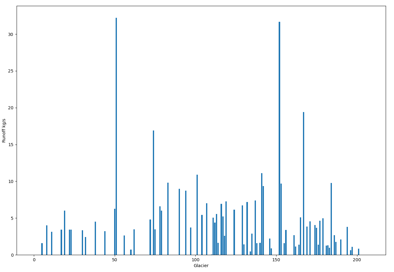
UM runoff interpolated onto 1km polar stereographic grid.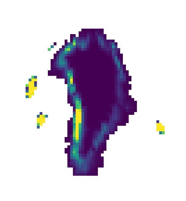
Drainage regions for each ocean facing glacier:

Figure: Drainage at each glacier
Thu 26 Jan 22:01:10 GMT 2023
Rignot data (ISMIP6)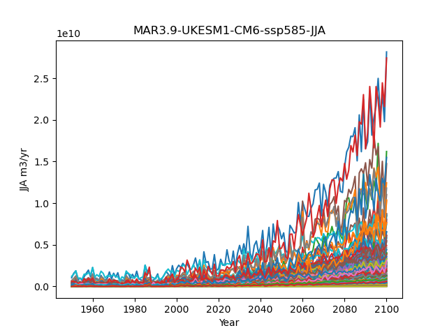
Tue 14 Feb 10:15:10 GMT 2023
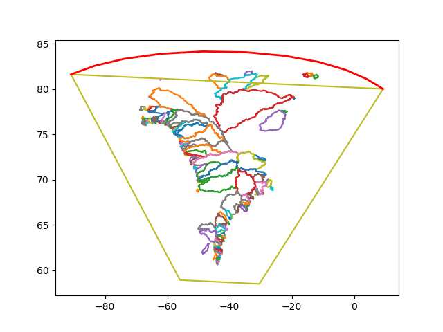
Recoding the drainage basin/UM coupling using polygon fraction overlap. The shapely Python library assumes flat domains. Is this OK for fractional overlap? Areas are obviously wrong, so using pyproj to calculate these in lat-lon space.No more regridding. Transforming polarstereographic (drainage) polygons into lat-lon space and calculating fractional overlaps with UM model grid.
Interesting (head hurting) effects of grid transfromation:
Figure: Runoff polygons transformed onto lat-lon grid
Wed 22 Feb 15:36:15 GMT 2023
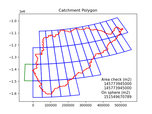
Catchment area intersect with (model) grid moxes. Algorithm finds matching boxes and calculates area contribution (flat space). Adjustment to area on sphere.Area check v1: area of catcmment. Area check v2: sum of contributed areas from model grid boxes.
Figure: polygon intersection with model grid
Wed 1 Mar 08:51:24 GMT 2023
Coastal fraction (UM model)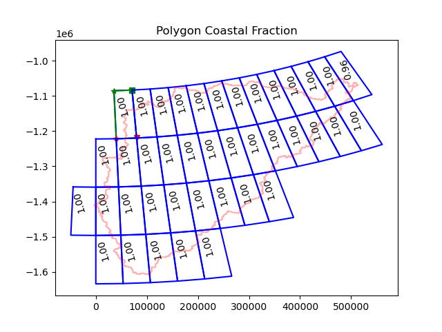
Thu 23 Mar 17:08:31 GMT 2023
UKESM meeting slides.Mask of Greenland bathymetry. Purple(!) above zero m. West coast drainage connection to central depressed region. Note, this is the high-res data from BedMachine.

Thu 13 Apr 21:51:21 BST 2023
Comparison of BISICLES calving flux with my calculated (potential) calving fronts.My fronts include floating ice and ice cells adjacent o open water.
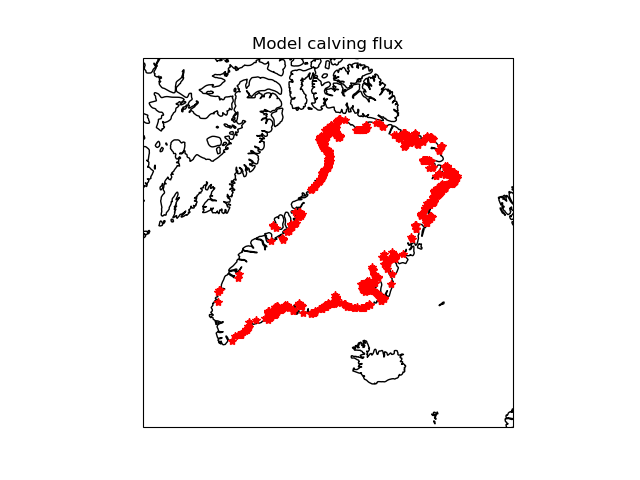
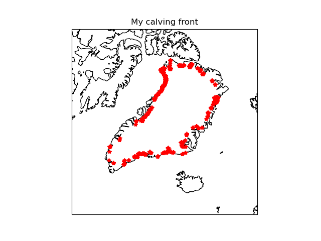
Fri 14 Apr 12:26:17 BST 2023
Bathymetry from model output zeroes out ocean area. Regrid BedMap2 (simply) onto required grid (NOTE: needed for ocean depth at ice front).
import cf
import numpy as np
from pyproj import Proj, Transformer
import cartopy.crs as ccrs
import matplotlib.pyplot as plt
from scipy.interpolate import RegularGridInterpolator

def get_farray(infile,field):
   fin=cf.read(infile)
   ma=fin.select(field)[0]
   dm=ma.data.array

   return dm

plt.ion()
inf4='zbase.nc'
tp=get_farray(inf4,'Z_base')


x_1d=np.load('x_1db.npy')
y_1d=np.load('y_1db.npy')

dx=x_1d[1]-x_1d[0]
dy=y_1d[1]-y_1d[0]


y_2d,x_2d = np.mgrid[y_1d[0]:y_1d[-1] + dy:dy, x_1d[0]:x_1d[-1] + dx:dx]

# GRIS projection
inProj= Proj('epsg:3413')
x0 = -654650.0
y0 = -3385950.0

x_2d2=x_2d+x0
y_2d2=y_2d+y0

plt.figure(20);plt.clf()
plt.imshow(tp)


infile='BedMachineGreenland-v5.nc'

fin=cf.read(infile)
bed=fin.select('bedrock_altitude')[0]
x=bed.dimension_coordinate('projection_x_coordinate').array
y=bed.dimension_coordinate('projection_y_coordinate').array # y.array
data=bed.data.array[::-1,:]
yy=y[::-1]
dx2=x[1]-x[0]
dy2=yy[1]-yy[0]
ya,xa=np.mgrid[yy[0]:yy[-1] + dy2:dy2, x[0]:x[-1] + dx2:dx2]


interp=RegularGridInterpolator((yy,x), data, bounds_error=False, fill_value=None)
new_dat=interp((y_2d2,x_2d2))

plt.figure(21);plt.clf()
plt.imshow(data)

plt.figure(22);plt.clf()
plt.imshow(new_dat)
plt.figure(23);plt.clf()
plt.imshow(new_dat-tp)
plt.figure(24);plt.clf()
plt.plot(new_dat[300,:],'r')
plt.plot(tp[300,:],'b--')
plt.show()
np.save('bathymetry',new_dat)


plt.figure(25);plt.clf()
plt.subplot(2,2,1)
plt.imshow(tp)
plt.title('Model Out')
plt.subplot(2,2,2)
plt.imshow(new_dat)
plt.title('Regridded Bedmap2')
plt.subplot(2,2,3)
plt.plot(new_dat[300,:],'r')
plt.plot(tp[300,:],'b--')
plt.title('Cross Section')
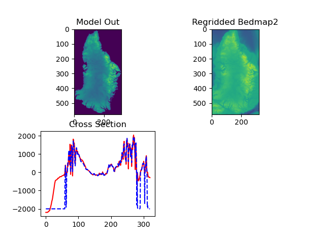
Calculated ocean depths at face:
Figure: Bathymetry at ice edge

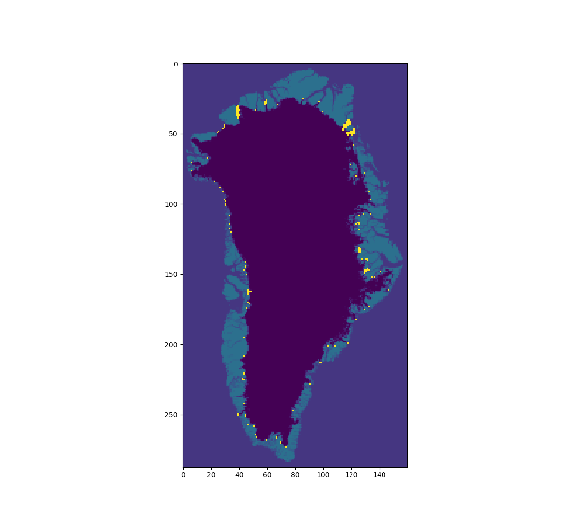
Thu 28 Sep 19:48:08 BST 2023
inSAR data verses BISICLES ice speed.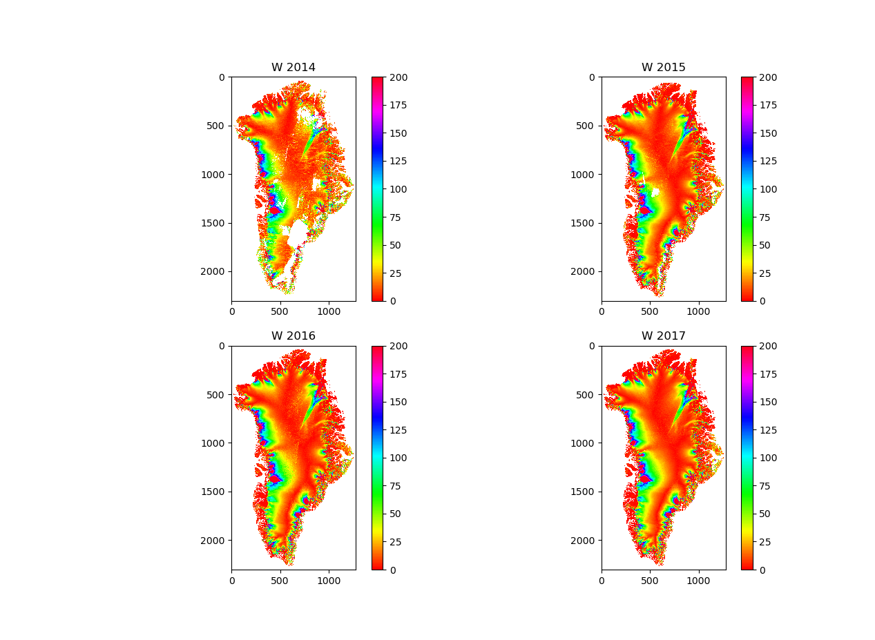
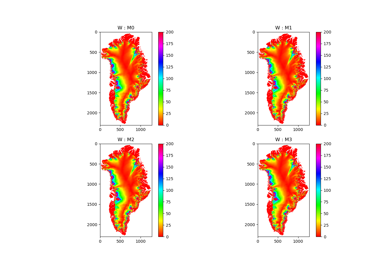
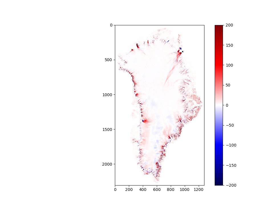
Glacier retreat after 50 years
Figure: Glacier retreat (yellow)
placer.