Python for IDL users
A guide for IDL users using Python for the first time. This web page is intended to help get you started using Python and making plots with Matplotlib. Please report any errors or ommisions to me - a.j.heaps@reading.ac.uk.
A more detailed look at Python is available on-line at Johnny Lin's website.
Setting up Python
To use the Canopy Enthought Python distribution in the Meteorology department type:
setup canopy
Users outside the department will need Python with the NumPy, matplotlib, basemap and netCDF4 packages installed.
Importing packages
In IDL all the functionality of the language is available by just typing idl - maps, stats etc. In Python you have to explicitly import packages you need. Some of the commonly used packages are:
import numpy as np - scientific computing
from scipy import interpolate - interpolation
import matplotlib.pyplot as plt - plotting
from mpl_toolkits.basemap import Basemap, shiftgrid, addcyclic - mapping
from subprocess import call - calling Unix programs
from netCDF4 import Dataset as ncfile - netCDF I/O
import cf - David Hassell's cf data I/O
After importing a package functions can then referenced - for example, np.mean(a) for the NumPy mean function.
Running Python programs
In Python no end statement or procedure/function name is needed. To run a Python program type
python prog.py
Python basics
Python floats are at least 64 bit numbers.
Python integers are 32 bit and not 16 bit as in IDL. A long integer is specified by putting a L or l after the number. Long integers can grow as large as is needed.
In Python variable names case sensitive while in IDL they are case insensitive. There is no need to declare variable types - just use them. As in IDL you can reassign variables to be different types.
# is the comment symbol. All text after a # is a comment.
Use print a,b,c to see the variables a,b,c. In IDL this would be print, a,b,c.
Array elements are accessed via [] brackets only. In IDL you can use both [] and (). Both Python and IDL indicies start at zero - i.e. the first element is a[0].
Indentation is the way of closing if then statements or loops in Python - there's no need for an endif or endfor as in IDL.
The rules of operator precedence are the same as in IDL - an integer multiplied by a float gives a float.
Python has a C style data interface while IDL has a Fortran style. If we have read in a standard atmosphere grid, in IDL it will appear as longitude, latitude, height, in Python it will appear as height, latitude, longitude. In IDL you would use a[i,*], the equivalent in Python is a[:,i]. See section on netCDF reading later.
Loops in Python
for i in np.arange(4):
  print i
0
1
2
3
Python is indentation sensitive so make sure your loop statements are indented. There is no end of loop statement in Python.
Large loops in Python are very slow. The following example is ten times slower than in IDL for a loop of 100 million points. A standard UM grid 96x73x22 for 360 days has 57 million points so this is not an unusual amount of data to be looking at.
First of all we create some test random data from -5 to 5. We will loop over the data and set the b array to be 1 for all points that are greater than zero.
a=np.random.rand(100000000)*10-5
b=np.zeros(100000000,dtype=int)
pts=np.arange(0,100000000)
for i in pts:
if a[i] > 0: b[i]=1
This took 160 seconds for a 100 million points.
Using pts=range(0,100000000) reduces this to 100 seconds.
Using NumPy where gives a much quicker answer
b=np.where(a < 0, a, 1) took 3.1 seconds
Using WHERE in IDL completed the same task in 0.16 seconds.
Creating arrays
The NumPy arange function is like INDGEN, FINDGEN in IDL. Up to three arguments are generally used - min, max and step. Note that result doesn't include the max value passed to it.
np.arange(5) - array([0, 1, 2, 3, 4])
np.arange(2,6) - array([2, 3, 4, 5])
np.arange(3,9,1.5) - array([3., 4.5, 6., 7.5])
Selecting data
a=np.arange(0,10,1) - array([0, 1, 2, 3, 4, 5, 6, 7, 8, 9])
a[0] - 0
a[-1] - 10
a[5:] - array([ 5, 6, 7, 8, 9, 10])
a[:5] - array([0, 1, 2, 3, 4])
The colon delimiter is used to indicate the beginning or end of a sequence. When used singly it means all values.
If / else examples
There are a variety of ways of doing an if statement in Python.
if condition:
  statements
else:
  statements
Python is indentation sensitive so make sure your statements are indented. There is no end of if statement in Python.
One line if commands are as follows:
if condition: do_something()
if condition: do_something(); do_something_else()
The following is also valid but more difficult to scan.
a = 1 if x > 15 else 2
Python conditionals
a == b Equal
a < b Less than
a > b Greater than
a <= b Less than or equal
a >= b Greater than or equal
a != b Not Equal
NumPy and Scipy documentation
The top level NumPy documentation is at
http://www.numpy.org
Scipy routine list is at
http://docs.scipy.org/doc/scipy/reference/index.html
For FFTs, regressions etc. look in the SciPy documenation.
Useful NumPy expressions
np.sqrt(a) - square root
np.log(a) - logarithm, base e (natural)
np.log10(a) - logarithm, base 10
np.exp(a) - exponential function
np.max(a), np.min(a), np.mean(a),
np.shape(a), np.ndim max, min, mean, shape, number
of dimensions of a.
These also take the axis=axis keyword to do function along an axis.
The first axis is axis=0.
np.pi - pi
np.nan - not a number
np.inf - infinity
To create a 3,5 array of np.zeros((3,5))+5
Averaging over axes:
np.mean(temp, axis=2) - note that axis=0 is the first axis
np.sum(temp, axis=1)
np.ceil(a) - round up
np.floor(a) - round down
np.int(a), np.float(a) - convert to integer, float
np.arange(5) - array([0, 1, 2, 3, 4])
Calendar functions
These are available via the
netcdftime module.
from netcdftime import utime
from datetime import datetime
cdftime = utime('hours since 0001-01-01 00:00:00')
print cdftime.units,'since',cdftime.origin
print cdftime.calendar,'calendar'
d = datetime(2006,9,29,12)
t1 = cdftime.date2num(d)
print t1
d2 = cdftime.num2date(t1)
print d2
hours since 1-01-01 00:00:00
standard calendar
17582028.0
2006-09-29 12:00:00
Passing data to routines and getting results back.
lonticks,lonlabels=mapaxis(min=plotvars.lonmin, max=plotvars.lonmax, type=1)
Define a routine with a def statement.
def myproc(min=min, max=max):
 return max-min
Don't forget to indent the lines after the procedure def line.
myproc(min=1, max=4) - 3
myproc(max=4, min=1) - 3
myproc(1,4) - 3 - this is using Python's keyword position to avoid putting in the min and max keywords.
To return multiple values return them comma separated with the return command
def myproc(min=min, max=max):
 return max-min, min+(max-min)/2.0
myproc(min=1, max=4) - (3, 2.5)
a,b=myproc(min=1, max=4)
Reading in netCDF data
Use the netCDF4 python interface.
from netCDF4 import Dataset as ncfile
nc=ncfile('gdata.nc')
lons=nc.variables['lon'][:]
lats=nc.variables['lat'][:]
p=nc.variables['p'][:]
temp=nc.variables['temp'][0,:,:]
: is a delimeter which here means all values. Python orders its data C style and IDL Fortran style. temp is a lon,lat,height grid and that's how it would appear in IDL. In Python it appears as height,lat,lon. In this example temp=nc.variables['temp'][0,:,:] gives the first value of pressure - 1000mb and all the longitudes and latitudes.
The data file - gdata.nc
Timing functions
To see where your code is spending the most time use the time module
import time
t1 = time.time()
do stuff
t2 = time.time()
print 'Time taken was ', t2-t1, 'seconds'
Python projects in the department
cf-Python - David Hassell's CF interface for reading, manipulating and writing data.
cfplot - The beginings of a simple contour / vector plotting package.
Making plots
Matplotlib is the basis for all the following plots. The code and data are available under each plot.
Basemap is used here for the map plots.
Graphs
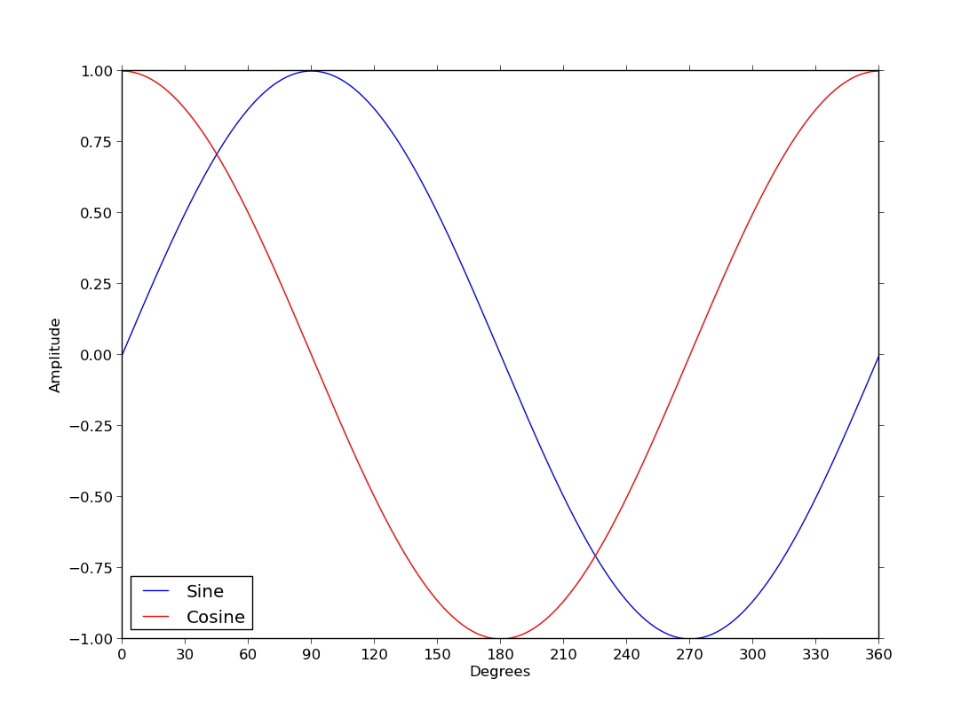
ex35.py
- sine and cosine curves and a legend
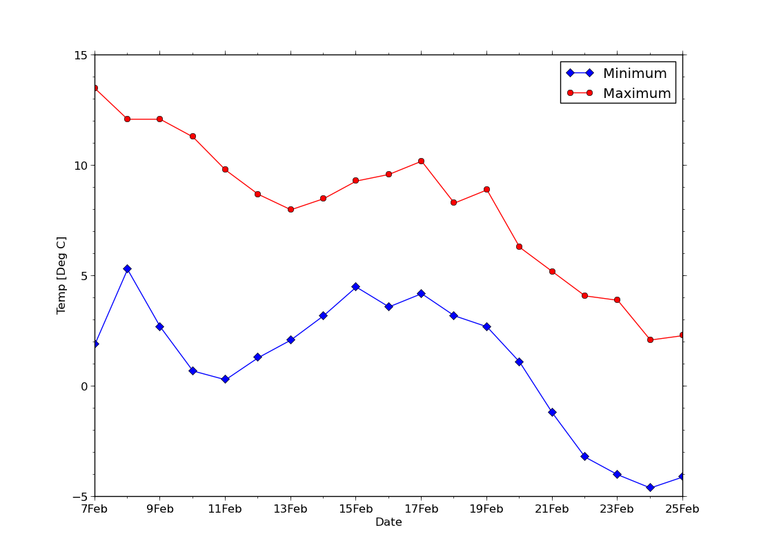
ex36.py
data
- lines with symbols, a non-numeric x-axis and minor tick marks
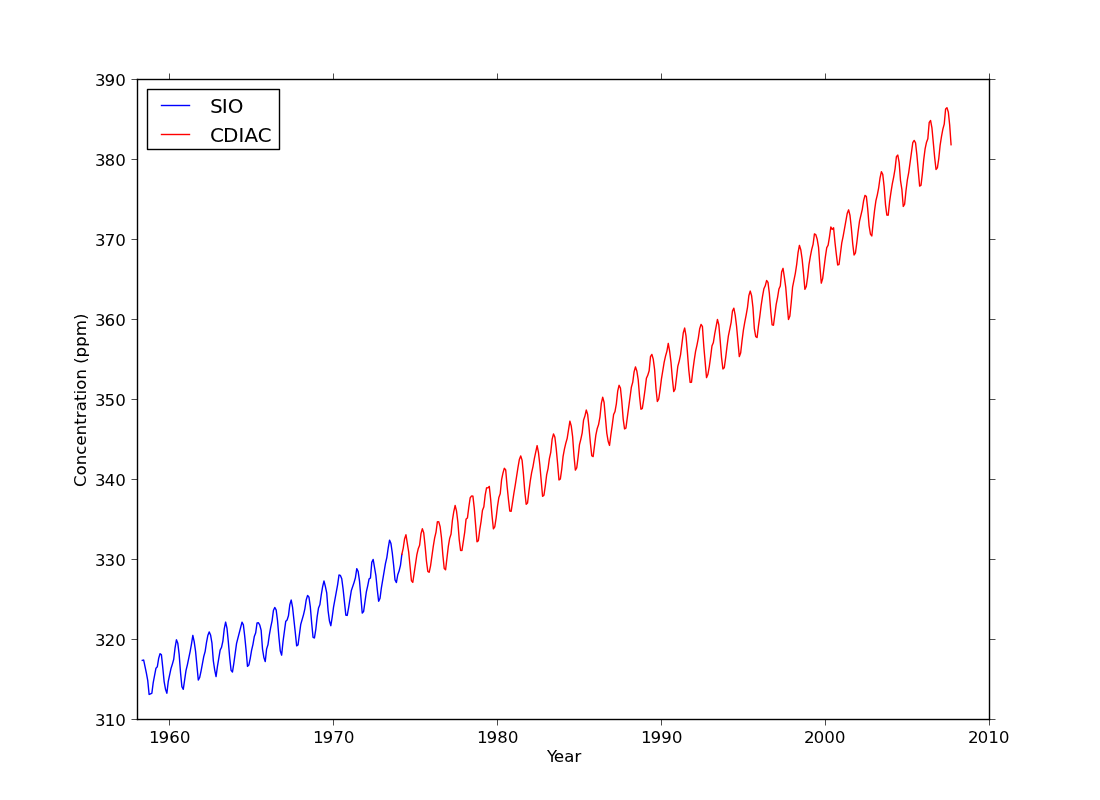
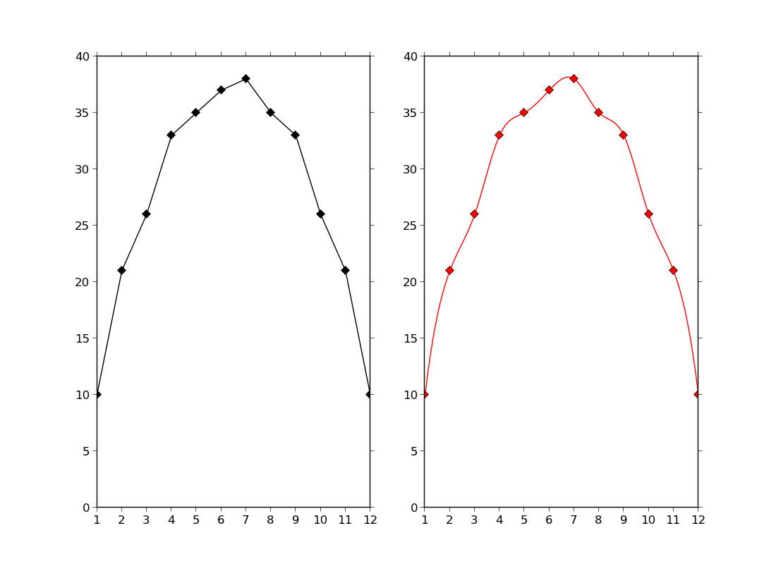
ex38.py
data
- one dataset but with two colours to represent different locations
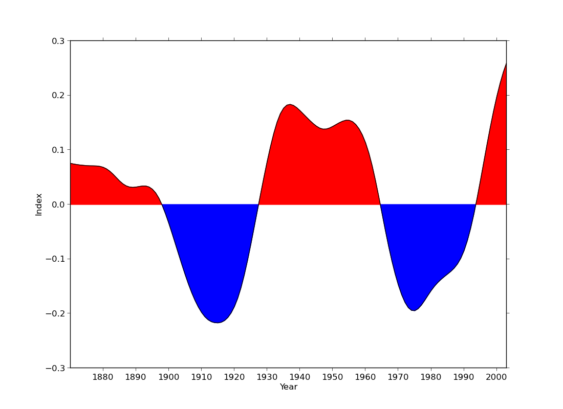
ex40.py
data
- filling a curve with colour
ex41.py
data
- graph with two y axes using twinx
ex43.py
- using cubic spline fitting from scipy
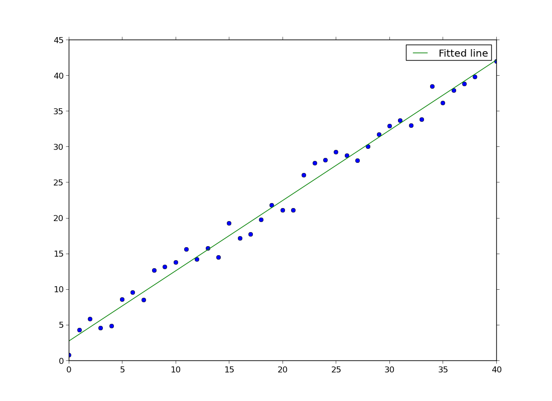
ex44.py
- line fitting
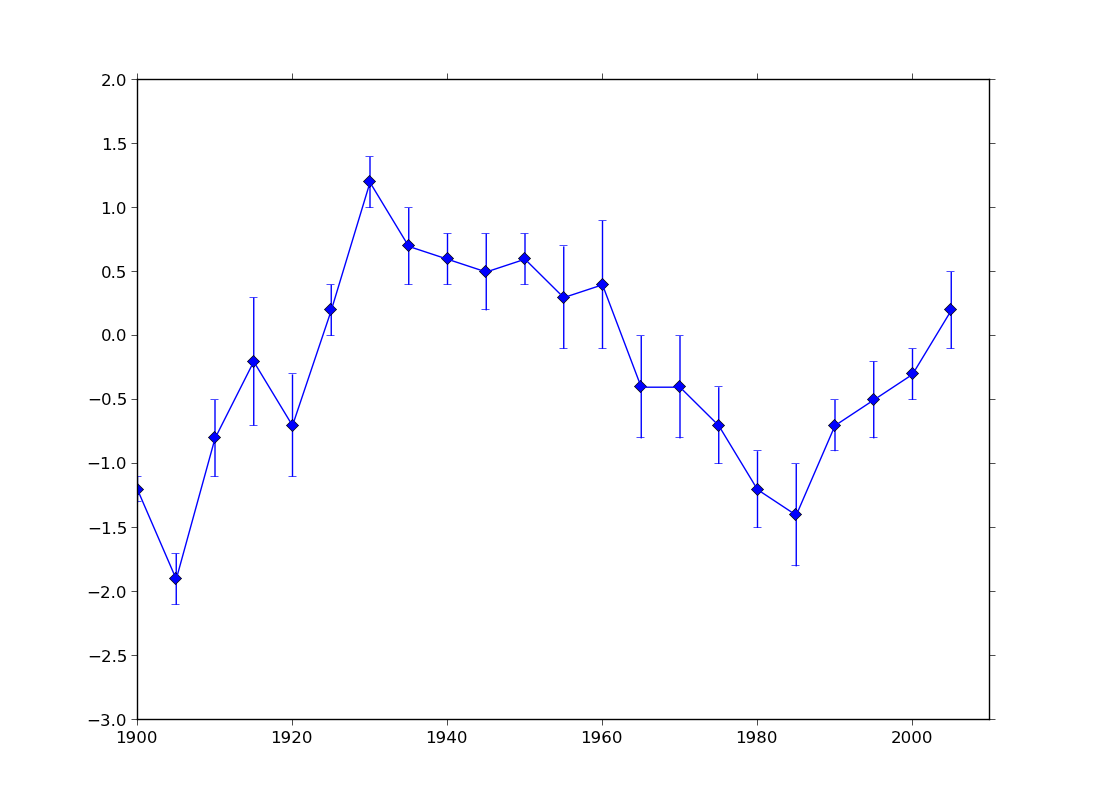
ex45.py
data
- error plot
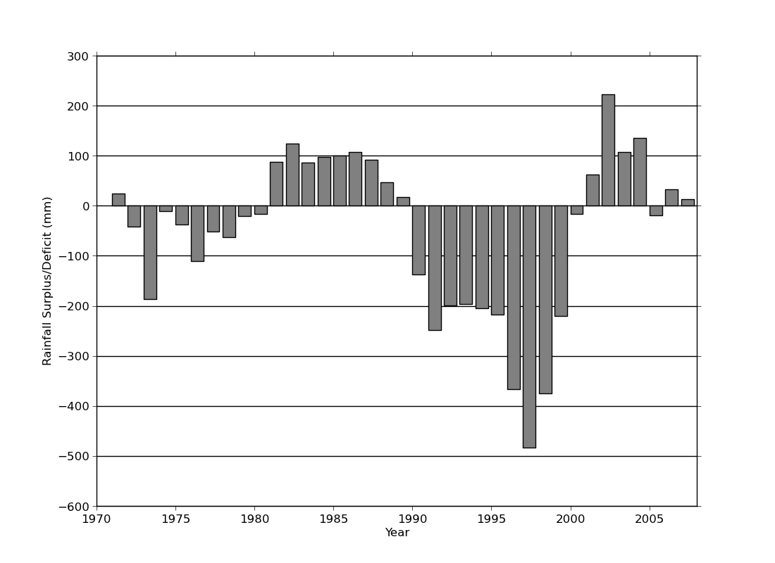
ex46.py
data
- bar plot. Horizontal lines behind bars were created using zorder=-1 to place them
behind all the plot elements.
Map contour plots
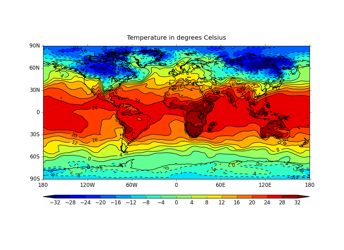
ex1.py
data
- colour contoured data on a cylindrical projection with a colour bar
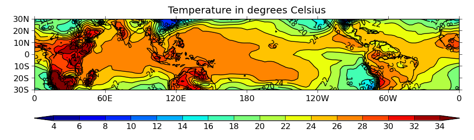
ex2.py
data
- zoomed version of the above
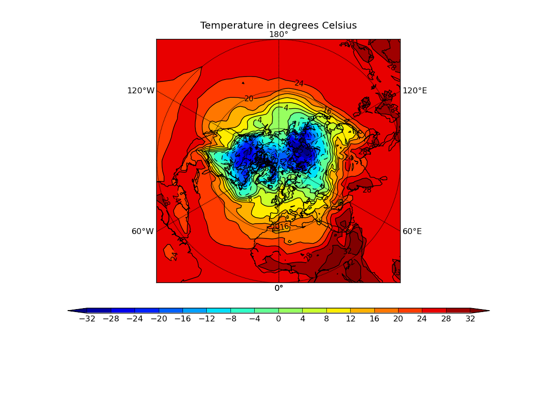
ex3.py
data
- northern hemisphere stereographic projection
ex4.py
data
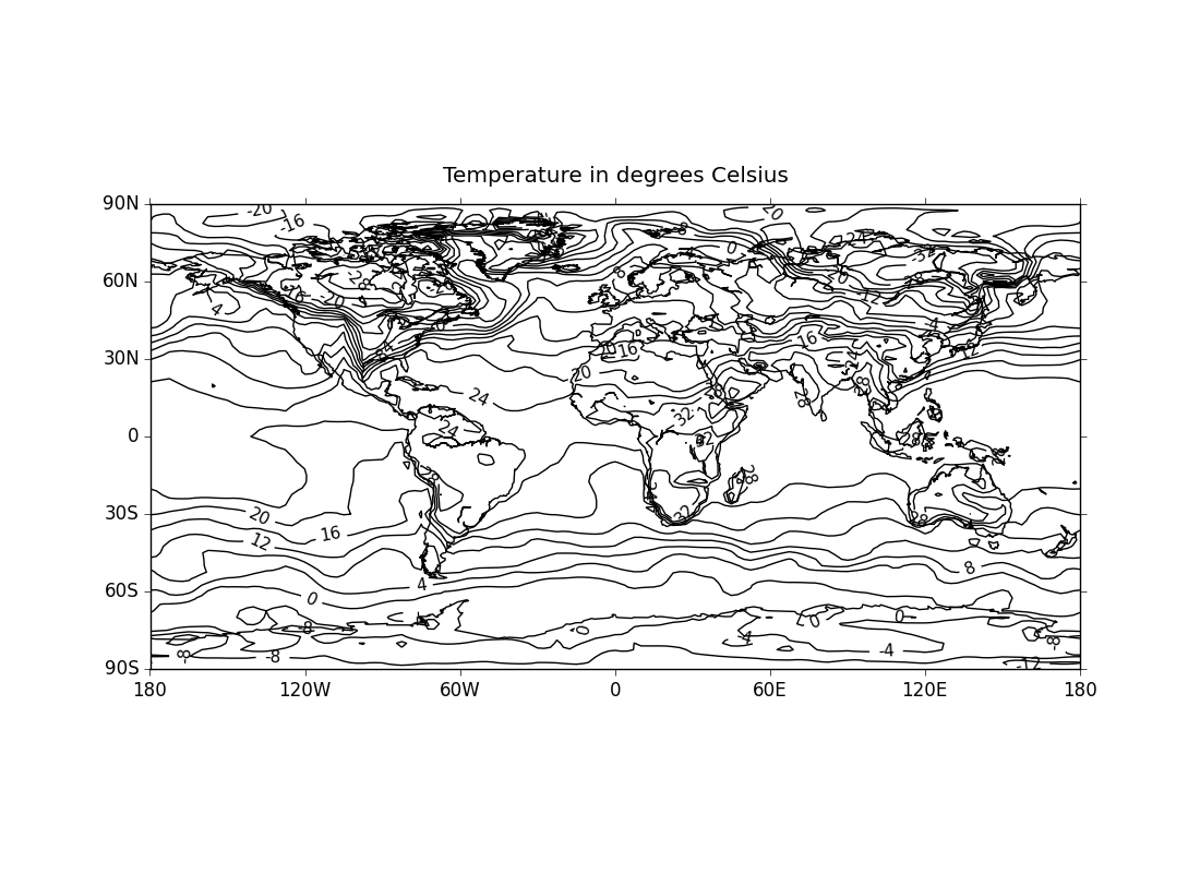
- unfilled contours with solid negative contour lines
ex5.py
data
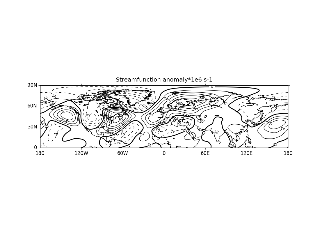
- thick zero contour line
ex28.py
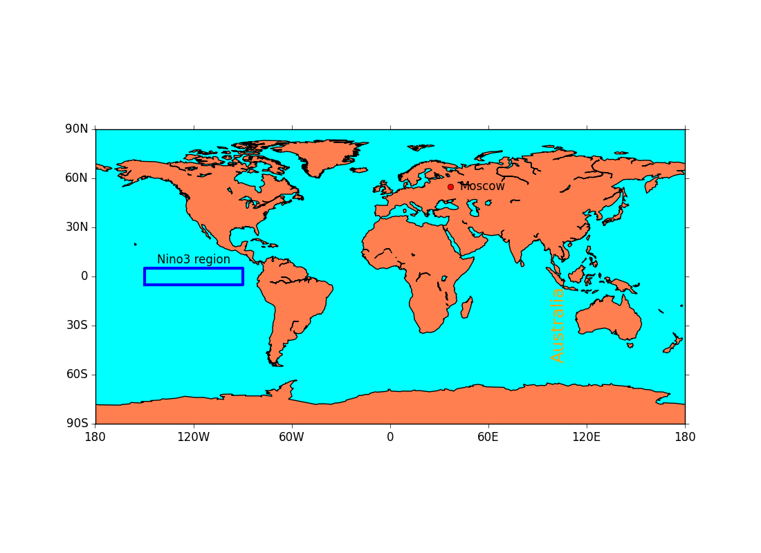
- drawing lines, text and symbols on a plot
Other contour plots
ex13.py
data
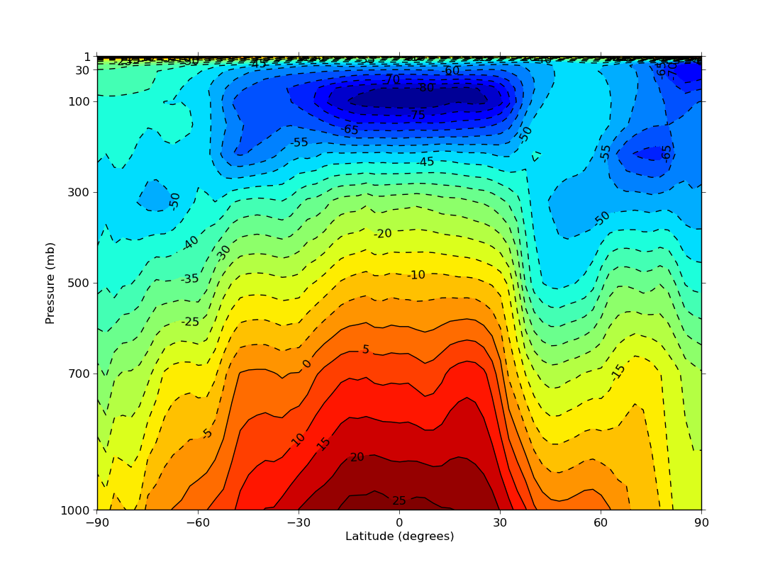
- linear pressure plot
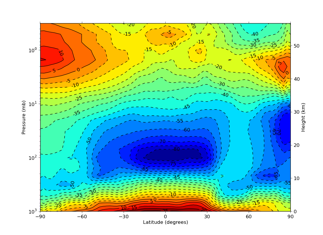
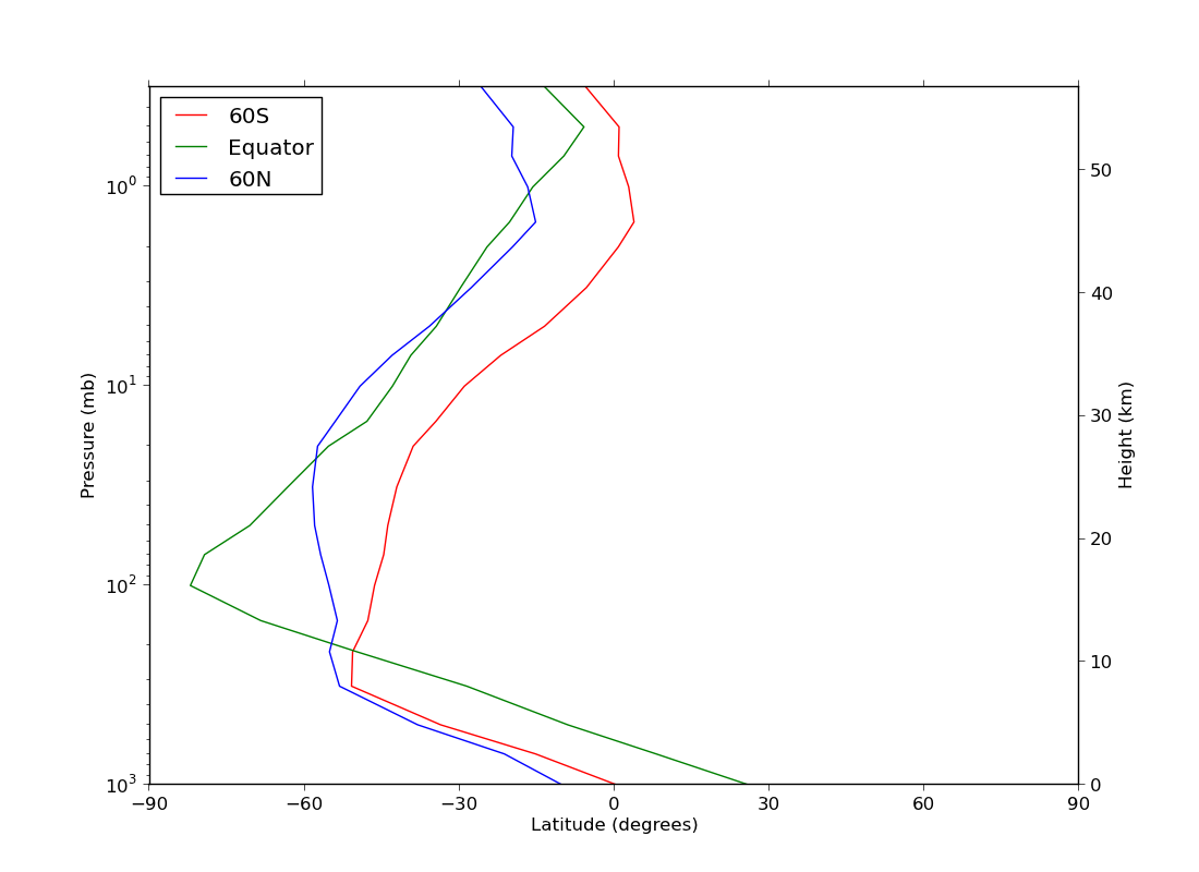
ex14.py
data
- log pressure plot with a both pressure and height labelled
y axes
Vector plots
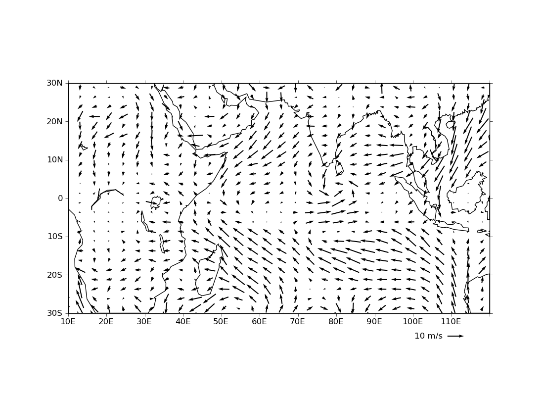
ex31.py
data
- vector plot with a key