Monday 25/01/2016

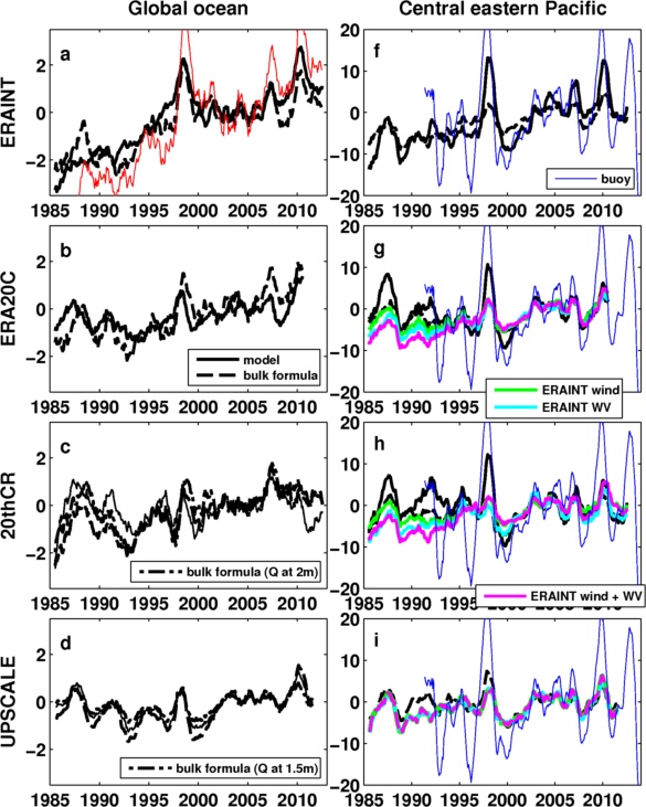
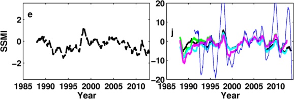
Fig. 1: The LH flux anomaly time series over the global ocean and central eastern Pacific (20^oN-20^oS, 210^oE-282^oE from different data sets.
from OAFLUX between two periods (2001-2008 minus 1986-2000). It shows mean negative trend over the central Eastern Pacific. The solid black box over the eastern Pacific is from 20^oN-20^oS and 210^oE to the west coast of Central America marked by Liu et al [2015]. The dashed box is from 8^oN-8^oS and 220^oE to the west coast of Central America where there are 27 buoy stations in it.

• All lines are 12 month running mean.
• In a-e, the solid line is model output, the dashed line is from bulk formula (Singh et al 2006) using SST, MSLP, wind and water vapour.
• The dot-dashed line uses dew point at 2m (for 2othCR) and 1.5m (UPSCALE).
• They are quite consistent over the global ocean.
• The red line in (a) is from COARE3.0 bulk formula. The trend is consistent with other two methods, but the variations are larger.
• (f-j) is over the central eastern Pacific, the blue line is from the TAO buoy stations in that box. Ther are 27 buoy stations in the box.
• The buoy data have higher variability. The mean for the buoys is simply the mean of all stations in the box.
• The green line is using ERAINT wind, thick cygn line uses ERAINT water vapour and the thick magenta line uses both ERAINT wind and water vapour.
• It seems the wind has larger effect on the trend.
• Need to check: in (i), 3 color lines nearly identical.
• Magenta line in (j) should be same as that of ERAINT.

Fig. 2: (a) is monthly buoy data points over central eastern Pacific. (b) is the composite LH flux anomaly from buoys. (c) is the LH flux anomaly time series from different data sets. The period means (1986-2000 and 2001-2008) are displayed in the plaot as well.

• There are good varibility consistency between data sets, particularly over 1997-2012.
• The buoy data show larger variability at the start and end.
• At the beginning, from 1990-1994, and in 2014, only a few buoys providing data.
• The peak arount 2012-2013 is outstanding.
• Both buoy data and OAFLUX show higher LH fluxes after 2000, but both model simulation show lower LH fluxes after 2000, consistent with what found.
• Since OAFLUX and ERAINT assimilated the buoy data, they are affected by the buoy data.
•            Over 2001-2004 and 2005-2008
• TAO buoy: -1.1    -0.4
• OAFLUX: 1.2    -1.0
• UPSCALE: 0.0    -1.2
• AMIP5 : 0.0    -2.11
• Buoy data still show increase trend.
• The mean LH flux changes over central eastern Pacific is much smaller than the mean flux variability.

Monday 18/01/2016

New plots

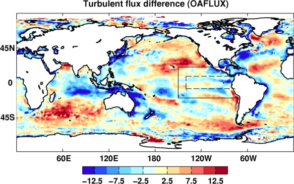
Fig. 1: The is LH flux difference from OAFLUX between two periods (2001-2008 minus 1986-2000). It shows mean negative trend over the central Eastern Pacific. The solid black box over the eastern Pacific is from 20^oN-20^oS and 210^oE to the west coast of Central America marked by Liu et al [2015]. The dashed box is from 8^oN-8^oS and 220^oE to the west coast of Central America where there are 27 buoy stations in it.

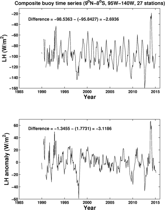
Fig. 2: Since data recorded at each buoy station have breaks and different starting time, we build a composite time series over the eastern Pacific (over the dashed box). The data are simply the mean of all stations in the box.

• There is a trend.
• The mean LH flux difference between the two periods are -2.7 and -3.1 W/m² for total flux and anomaly respectively.

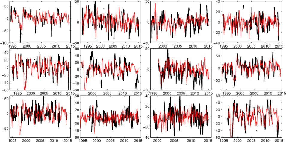
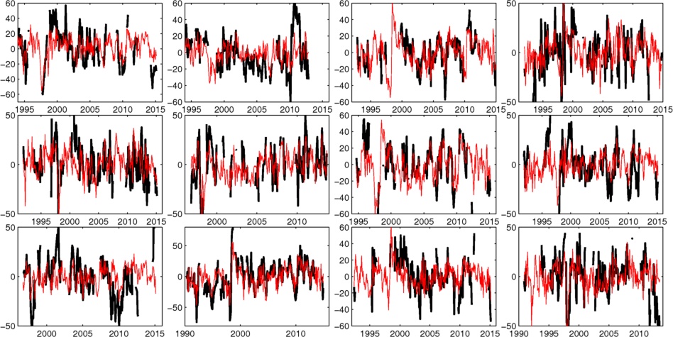
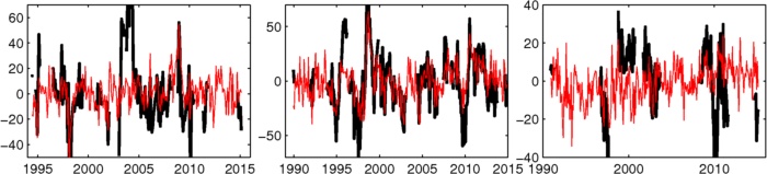
Fig. 3: Anomaly time series at each of 27 buoy stations in the dashed box of central Eastern Pacific.

• Some stations have the negative trend.
• Most stations show flat time series.
• In general, it doesn't give much information. The composite one is more useful.
• They are shown here for reference only.

Wednesday 13/01/2016

Surface tubulent flux comparison with buoy data

After reconstruction of TOA (top of atmosphere) radiation fluxes (F_T) [Allan et al. 2014], the surface net energy fluxes are estimated by Liu et al. [2015] combining F_T and the atmospheric energy transport (divergence) from ERA-Interim atmospheric reanalysis [Dee et al. 2011; Berrisford et al. 2011] (hereafter ERAINT).

The estimated surface fluxes need to be cross checked with other data sets derived using different methods, particularly with "observations", such as flux data from object analysis (OAFLUX [Yu et al ????]) and buoy stations.

This study focus on the turbulent flux comparison and it includes two parts:

• (1) due to the discrepancy of total column water vapor content in ERA-Interim reanalysis and satellite observations, the surface fluxes are corrected using observed total coloumn water vapour content (W) from satellite observations of SSM/I and SSMIS (hereafter SSMI).
• (2) the surface turbulent fluxes (before and after the W corrections and they are noted as W_B and W_A, respectively) are calculated by removing the surface radiation fluxes of CERES from our estimated net surface flux [Liu et al 2015]. The turbulent fluxes are compared with those from OAFLUX and buoy stations (RAMA, TAO and PIRATA).

• All data are monthly mean data.
• Derived surface turbulent fluxes : before and after the W corrections (W_B and W_A).
• OAFLUX data are used for comparison.
• Buoy station turbulent fluxes : TAO (68 stations), RAMA(26 stations), PIRATA (20 stations).
• The details of the W correction is at the site of https://www.met.reading.ac.uk/~sgs01cll/WV/wv.html (section : Friday 11/12/2015).
• Unless stated, otherwise the data period is from Mar 2000 - Feb 2015 (compatable with the CERES period).
• The downward turbulent flux is defind as positive.
• The bias and root mean squared error (RMSE) are deined as:

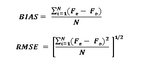
where N is the total data points, F_e is the estimated flux and F_o is the observed flux.

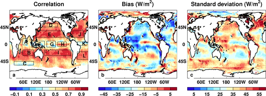
Fig. 1: Spatial distribution of (a) correlation coefficient, (b) bias and (c) RMSE. They are all calculated from turbulent flux anomalies between W_B and OAFLUX.

• Similar results are obtained if W_A data are used).
• The data period is from Mar 2000 - Feb 2015. It is also the BASE period for anomaly calculations.
• The correlaton coefficients are high in general, but there are low correlations around tropics and the southern end of Indian Ocean.
• The interested areas of different correlation coefficients are marked from A to L, which will be investigated futher next.
• There is a systematic bias between W_B and OAFLUX. The mean bias over the global ocean is about -19W/m².
• The mean turbulent fluxes over the oceans covered by the OAFLUX data are -124 (-122), -124 (-122) and -105W/m² for W_B, W_A and OAFLUX respectively.
• They are means from Mar 2000 - Feb 2005. The value in the bracket is over the global oceans.
• Meanwhile the mean turbulent flux over the global ocean is 116W/m² from Wild et al (2015) over 2000-2005.
• The RMSE is generally high, particularly over western Pacific and north Atlantic, consistent with the systematic biases over these areas.

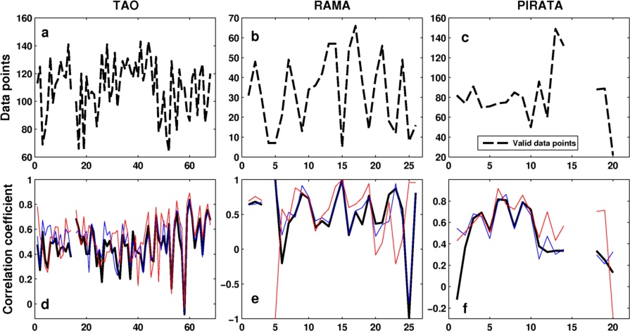
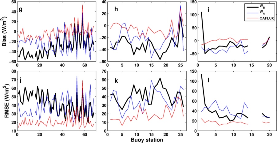
Fig. 2: Statistics of comparisons of turbulent fluxes between W_B, W_A, OAFLUX and buoy stations.

• For comparison with the buoy data, the grid point nearest to the buoy station is chosen from W_B, W_A and OAFLUX data sets.
• Most of the long records are from TAO data set and a few from PIRATA data set. The RAMA data only cover a few years.
• Since there are breaks in the buoy data time series, the data points are used for the calculations wherever the bouy data points are valid, in order to avoid bias.
• The correlation coefficeints are calculated from anomalies. The seasonal climatology is based on the valid datapoints of the buoy data between Mar 2000 - Feb 2015.
• The correlation coefficeints are quite consistent over TAO buoys for three data sets.


• The bias is mean difference between two time series at each station.
• Since the OAFLUX data are 'OA' (object analysis) data from observations, so its mean bias is near zero.
• For W_B and W_A, there are quite big systematic mean biases as discussed above.
• For TAO data, after W correction, the bias is a bit smaller.
• For PIRATA station 1, there is a large anomaly before W correction. (need checking)
• The RMSE is also large.

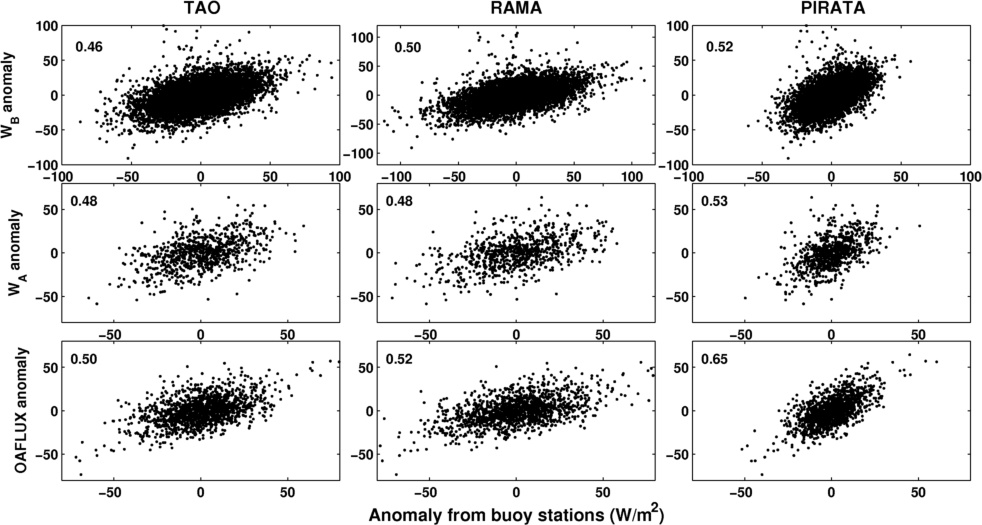
Fig. 3: Scatter plot of turbulent flux anomalies. The anomalies are collections of individual anomaly time series from each buoy stations.

• The correlation coefficient is from 0.46 to 0.65.
• W_B, W_A, and OAFLUX are all performed well, but W_B gives larger anomalies.
• The correlation coefficient of OAFLUX with buoy data is slightly higher.

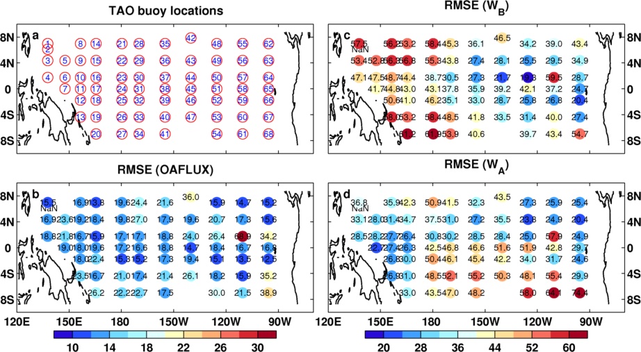
Fig. 4: (a) TAO buoy station locations, (b) RMSE (between OAFLUX and buoy data), (c) RMSE (between W_B and buoy data), (d) RMSE (between W_A and buoy data).

• This data set covers 8^oN-8^oS of Pacific.
• There are larger discrepancies at station 57 and 68.
• For W_B, there are larger discrepancies over west central Pacific than that over eastern Pacific.
• For W_A, larger discrepancies are over the south of the Eqator.

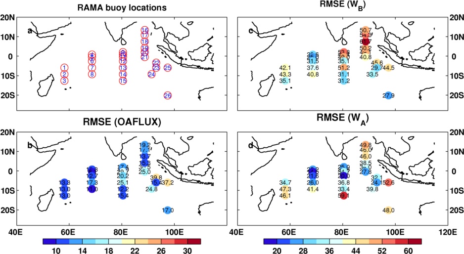
Fig. 5: As Fig. 4, but for RAMA data in Indian Ocean.

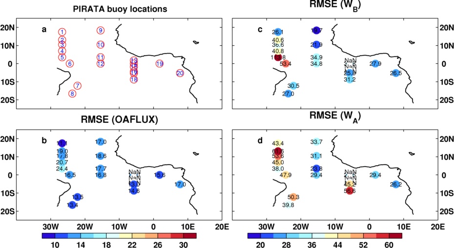
Fig. 6: As Fig 4, but for PIRATA data in central Atlantic.

• Note: the map is not right.

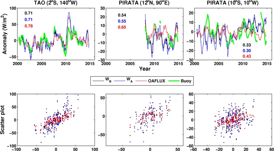
Fig. 7: Top row is the anomaly time series at three buoy stations, and the lower row is their corresponding scatter plot.

• TAO has longest record in general.
• The reference period for each buoy station varies due to different record length. Foe each station, the data points used for seasonal climatology is the same as those in the buoy record.
• The correlation coefficients between W_B, W_A, OAFLUX and buoy data are displayed in the plots.
• Correlation coefficients from three data sets are consistent, but OAFLUX gives slight high values.
• Lines are six month running mean.

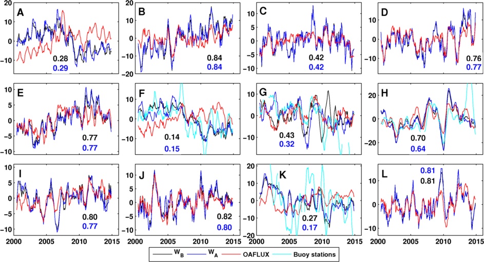
Fig. 8: Area mean turbulent flux anomaly time series.

• Area A-L are marked in Fig. 1.
• Lines are six month running mean.
• Climatology period Mar 2000 - Feb 2015.
• Means from W_B, W_A and OAFLUX are area weighted means. The means from buoy stations are just the mean of the data in the area box.
• Only buoy data over area F, G, H and K are used since there are more buoy stations in those area boxes.
• Over area F, the correlation between W_B and buoy data is 0.61, much higher than that between OAFLUX and buoy data (0.28 as shown in the table below).
• The correlation coeffcients are comaprable over area G, H and K.


• The correlation coeffcients are displayed in the plots. black values are between W_B and OAFLUX, blue values are between W_A and OAFLUX.
• The correlation coeffcients with buoy data over area F, G, H and K are listed in table below.

Table 2: Correlation coeffcients between W_B, W_A, OAFLUX and buoy station data.

Area	Number of buoy stations	WB	WA	OAFLUX
F	12	0.61	0.51	0.28
G	21	0.43	0.42	0.44
H	15	0.40	0.36	0.34
K	5	0.22	0.24	0.19

• Our estimated turbulent fluxes (W_B and W_A) have high correlations with OAFLUX data over the oceans, except those over the tropics.
• There are systematic biases between our estimates and OAFLUX and buoy data.
• Regarding to the correlations, our estimates are comparable with OAFLUX.
• Over region F, our estimates have higher correlations with buoy data than OAFLUX.

Through the comparison with observations, though there are systematic biases between our estimates and observations, there are very good correlations in the variability. The effect of total column water vapor content correction on the derived products is small.