2. The CFA framework

2.1. A conceptual framework for the in-memory storage of aggregated arrays

A master data array is one which is constructed from the one or more sub-arrays.

The simplest master data array has just one sub-array which is equal to itself, but in general, a master data array may have up to as many, non-overlapping sub-arrays as is it has elements and each sub-array contains a contiguous subset of the master data array values. See figure 1a and figure 2a for examples of master data arrays and their constituent sub-arrays.

A master data array constructed from sub-arrays arises naturally from an aggregation process, such as by the CF aggregation rules.

Sub-arrays may be be combined to create hyperrectangular [1] master data arrays, which poses storage and access difficulties since there may be different numbers of sub-arrays across different sections of the same master data array dimension. For example, the master data array in figure 2a has three sub-arrays spanning the first two rows (values 0 to 6 and 7 to 13) but only two sub-arrays spanning third row (values 14 to 20). Such an irregular construction would, for example, complicate finding which sub-array contained a particular element or, more importantly, complicate the recombination of sub-arrays into an equivalent master data array (an operation required by the CF aggregation process).

A solution is to decompose the master data array into a hyperrectangular partition matrix such that its elements (called partitions) span all or part of exactly one sub-array. A given partition’s data array is then a reference to a unique part of a unique sub-array. See figure 1b, figure 1c and figure 2b for examples.

The master data array may be therefore be considered as being constructed from a hyperrectangular matrix of partitions. See example 1 and example 2.

A guaranteed hyperrectangular decomposition renders easy any operations requiring knowledge of the partition locations within the master data array (such as element location or partition matrix transposition) and allows the master data array to be aggregated with other master data arrays.

2.2. Larger-than-memory arrays

Sub-arrays larger than the available memory may be stored effectively in memory by simply ensuring that such a sub-array is kept in a file and partitioning the master data array so that each partition is small enough to be realized in memory, if required.

2.3. Subspaces

A subspace of a master data array may be created easily by discarding partitions which do not overlap the subspace and for each remaining partition, adjusting the definition of the part of the sub-array which comprises the partition’s data array (see the part parameter).

2.4. Partition matrix properties

• The partition matrix’s dimensions are always a subset of the master data array’s dimensions. I.e. each dimension of partition matrix index space corresponds to a dimension of the master data array.
• The partition matrix may be a scalar, if it contains exactly one partition whose data array spans the entire master data array.
• The partition matrix may span fewer dimensions than the master data array (see figure 1b, in which the partition matrix is 1-dimensional but the master data array is 2-dimensional), but never more.
• The order of the partition matrix’s dimensions may be different to the relative ordering of the equivalent dimensions of the master data array.
• The creation of a subspace of the master data array may result in one or more partitions which reference a non-contiguous part of a sub-array (see the part parameter).

2.5. Examples

2.5.1. Example 1

The 2-dimensional 2 x 7 master data array in figure 1a is composed from 3 sub-arrays. The most efficient way of partitioning the master data array into a hyperrectangular partition matrix such that each partition contains all or part of exactly one sub-array is shown in figure 1b. Note that, in this case:

• The partitions’ data arrays are not all of the same size or shape
• Each partition’s data array spans an entire sub-array
• The partition matrix has fewer dimensions than the master data array.

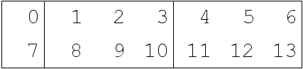
Figure 1a. The 3 sub-arrays of the master data array.

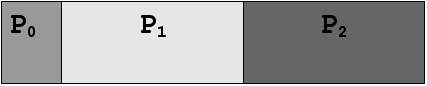
Figure 1b. A 1-dimensional, 3 element partition matrix of the master data array. Each block of colour represents one of the 3 sub-arrays and each partition of the partition matrix is labelled P_x. For example, the partition data array of P₀ contains values 0 and 7.

Another, equally valid partitioning of the master data array is shown in figure 1c. Note that, in this case:

• No partitions’ data arrays span an entire sub-array.
• The partition matrix has the same number of dimensions as the master data array.

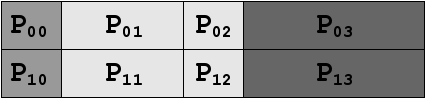
Figure 1c. A 2-dimensional, 2 x 4 element partition matrix of the master data array. Each block of colour represents one of the 3 sub-arrays and each partition of the partition matrix is is labelled P_yx. For example, the partition data array of P₁₁ contains values 8 and 9 and the partition data array of P₁₂ contains value 10.

2.5.2. Example 2

The 2-dimensional 8 x 7 master data array in figure 2a is composed from 10 sub-arrays. The most efficient way of partitioning the master data array into a hyperrectangular partition matrix such that each partition contains all or part of exactly one sub-array is shown in figure 2b. Note that, in this case:

• The partitions’ data arrays are not all of the same size or shape
• Some partitions’ data arrays span an entire sub-array (P₀₀ and P₃₃), but the rest do not.

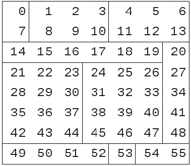
Figure 2a. The 10 sub-arrays of the master data array.

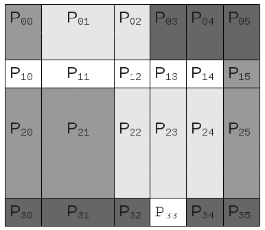
Figure 2b. A 2-dimensional, 4 x 6 element partition matrix of the master data array. Each block of colour represents one of the 10 sub-arrays and each partition of the partition matrix is labelled P_yx. For example, the partition data array of P₃₀ contains value 49; the partition data array of P₃₁ contains values 50 and 51; and the partition data array of P₃₂ contains value 52.

2.6. Accounting for arbitrary partition data array properties

There are properties of a partition’s data array which are arbitrary in the sense that, whilst these properties may differ to their equivalents in the master data array, the partition’s data array may always be altered to conform with the master data array with no loss of information.

A partition’s data array inherits these properties, unchanged, from the sub-array which contains it.

The properties for which a partition’s data array may differ from its master data array are:

• The order of dimensions.
• The number of size 1 dimensions.
• The sense in which dimensions run.
• The units of the data values.
• The missing data value.

When a partition’s data array is required by the master data array, it needs to be conformed by doing any or none of:

• Reordering its dimensions to the same order as the master data array.
• Removing size 1 dimensions which don’t exist in the master data array.
• Adding size 1 dimensions which exist in the master data array but not in the partition’s data array.
• Reversing dimensions which run in the opposite direction to the master data array.
• Converting the data values to have the same units as the master array.
• Either the missing data value is converted to that of the master array (accounting for conflicts with non-missing data values) or, if arrays are stored with ancillary missing data masks (as can be the case with python numpy arrays, for example), the partition’s data array’s missing data value may be ignored.

2.7. Parameters required for specifying a master data array

It follows that a master data array and its partitions may be completely specified by a small number of parameters.

Note

When a partition has a parameter value equal to the master array then there is some redundancy which will be exploited when storing the array by its parameters with the CFA-netCDF conventions.

2.7.1. Master data array parameters

The master data array comprises:

dtype

The data type of the master data array.

units

The units of the master data array.

calendar (if required by units)

The calendar of the master data array.

dimensions

An ordered list of the master data array’s dimensions.

shape

An ordered list of the master data array’s dimension sizes. The sizes correspond to the dimensions list.

Partitions

A matrix of the master data array’s partitions. Each partition is described by its partition parameters.

2.7.2. Partition matrix parameters

pmdimensions

An ordered list of the dimensions along which the master data array is partitioned. Each of these dimensions is one those specified by the dimensions parameter.

pmshape

An ordered list containing the number of partitions along each partitioned dimension of the master data array. The sizes correspond to the pmdimensions list.

2.7.3. Partition parameters

Each partition of the partition matrix comprises:

pdimensions

An ordered list of the partition’s data array dimensions.

punits

The units of the partition’s data array.

pcalendar (if required by punits)

The calendar of the partition’s data array.

flip

A collection of the partition’s data array dimensions which run in the run in the opposite direction to those of the master data array.

location

An ordered list of ranges of indices, one for each dimension of the master data array, which describe the contiguous section of the master data array spanned by this partition. The ranges correspond to the dimensions list.

part

An ordered list of indices for each dimension of the partition’s data array which describe the part of the sub-array which is spanned by this partition. The indices correspond to the pdimensions list.

subarray

A reference to the sub-array which contains the partition’s data array.

---

Footnotes

[1]	The generalization of a rectangle for higher dimensions.