PHYS 8.3: Multi–electron atoms |
PPLATO @ | |||||
PPLATO / FLAP (Flexible Learning Approach To Physics) |
||||||
|
1 Opening items
1.1 Module introduction
The hydrogen atom has a beautiful simplicity – it comprises a single electron moving around the nucleus and it therefore has the simplest structure of all atoms. By focusing their attention on this atom, the scientists of the late nineteenth and early twentieth centuries were able to make substantial progress in understanding atomic structure in general. The Bohr model for atomic hydrogen was a key stage in this study.
Atoms that are heavier than hydrogen, the so–called multi-electron atoms, are rather more difficult to understand. This module examines some of the methods used to investigate these atoms and introduces some of the laws that govern their structure.
Most experiments on multi–electron atoms involve transferring energy to or from them. If sufficient energy is supplied, electrons can be removed. Although the energy needed to remove successive electrons from an atom generally increases as the number of remaining electrons decreases, it does not do so in a regular way. The pattern of these successive ionization energies suggests that the electrons are contained in groups (electron shells) at various mean distances from the central nucleus.
Subsection 2.2 describes the technique of photoelectron spectroscopy which can be used to explore the arrangement of electrons in more detail. Photoelectron spectroscopy shows that the energy levels that compose each electron shell are themselves grouped together in subshells of very similar energy. Subsection 3.1 describes some empirical rules for working out the maximum number of electrons that may be found in any particular shell or subshell; Subsection 3.2 introduces the s-p-d-f notation for labelling subshells which allows us to write the electronic configuration of an atom in a convenient shorthand way (Subsection 3.3).
Section 4 explains the origin of the empirical rules introduced in Section 3. In order to do this it uses some of the ideas that underpin the quantum model of the atom developed in the 1920s. The full mathematical formalism of quantum theory is not used, but some of its results are quoted along with some of the experimental evidence that supports them, such as the Zeeman effect (which demonstrated the quantization of orbital angular momentum) and the Stern–Gerlach experiment1 (which demonstrates the quantization of spin angular momentum). Using these ideas, Subsection 4.5 describes the way in which each of the electrons in an atom can be characterized by the values of four quantum numbers: the principal quantum number n, the orbital angular momentum quantum number l, the orbital magnetic quantum number ml, and the spin magnetic quantum number ms. The values of these quantum numbers are related to the energy of the electron. Subsection 4.5 also leads to the Pauli exclusion principle, the requirement that no two electrons shall have the same values for all four quantum numbers, and shows how this leads to the observed distribution of energy levels. This in turn, together with Hund’s rule, explains the observed ground state electronic configurations of the various chemical elements.
Finally, in Section 5 the origins of continuous and characteristic X–ray spectra are described, along with their historical role in revealing the natural sequence of elements according to atomic numbers.
Study comment Having read the introduction you may feel that you are already familiar with the material covered by this module and that you do not need to study it. If so, try the following Fast track questions. If not, proceed directly to the Subsection 1.3Ready to study? Subsection.
1.2 Fast track questions
Study comment Can you answer the following Fast track questions? If you answer the questions successfully you need only glance through the module before looking at the Subsection 6.1Module summary and the Subsection 6.2Achievements. If you are sure that you can meet each of these achievements, try the Subsection 6.3Exit test. If you have difficulty with only one or two of the questions you should follow the guidance given in the answers and read the relevant parts of the module. However, if you have difficulty with more than two of the Exit questions you are strongly advised to study the whole module.
Question F1
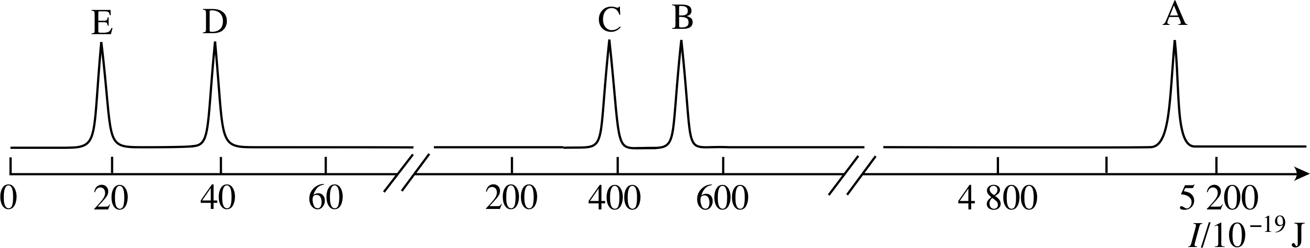
Figure 1 See Question F1.
Figure 1 is the photoelectron spectrum of argon gas, which consists of single atoms. What evidence is contained in this spectrum for the existence of electron shells and subshells? Sketch an electron energy level diagram for argon. i Label the levels with values of the principal quantum number n and the appropriate letter to denote the orbital angular momentum quantum number l.
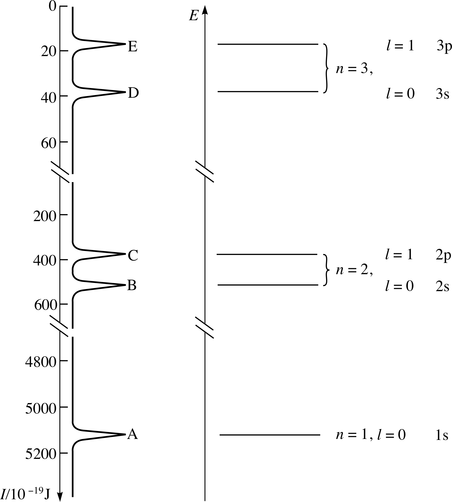
Figure 23 See Answer F1.
Answer F1
The production of photoelectrons with discrete energies (each of which corresponds to one of the five peaks) shows that the electrons in the atom have discrete energies. The ionization energies of argon fall into three groups: A; B and C; D and E. This indicates that there are three shells occupied by electrons in the argon atom. In the two outermost shells, the presence of more than one peak in the photoelectron spectrum shows the existence of subshells.
An electron energy level diagram for argon can be obtained simply by turning the photoelectron spectrum clockwise through 90° (Figure 23). Each peak in the spectrum corresponds to a subshell that contains at 4800 least one electron; the highest threshold energy I corresponds to the innermost electrons.
In the electron energy level diagram (as in the spectrum) the levels are arranged in groups. These groups are the electron shells, which are labelled with the principal quantum number n. This quantum number has integral (whole-number) values from 1 up to 3 (Figure 23).
Within the shells, the existence of subshells is revealed by the closely spaced peaks within each group in the photoelectron spectrum. The subshells are labelled with a second quantum number l, which can take any integer value from zero to n − 1. The l values 0, 1, 2, 3 are represented by the letters s, p, d, f, respectively.
Question F2
State the values of all the quantum numbers for each of the six 2p electrons in an atom.
Answer F2
All six have n = 2 and l = 1. See Table 3 for the other quantum numbers.
Question F3
Write down, in the standard notation, the electronic configuration of a rubidium atom in its ground state. (The atomic number of rubidium is 37, and its chemical symbol is Rb.)
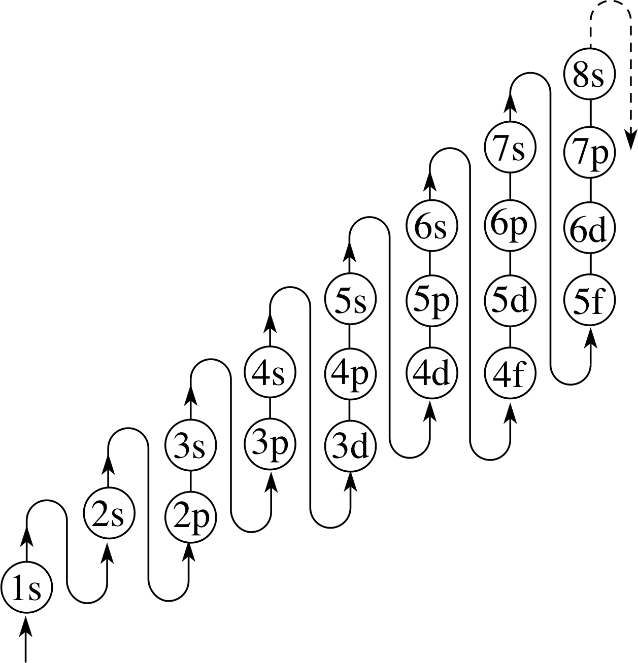
Figure 19 The order in which the subshells are filled for atoms in their ground states.
Answer F3
Referring to the ‘snake’ in Figure 19, the order in which the subshells will be filled is 1s, 2s, 2p, 3s, 3p, 4s, 3d, and so on.
The electronic structure of rubidium in the ground state is therefore:
Rb 1s2 2s2 2p6 3s2 3p6 4s2 3d10 4p6 5s
Question F4
To what extent is the emission of characteristic X–rays by multi–electron atoms analogous to the emission of visible spectral lines by hydrogen atoms?
Answer F4
The analogy is very close. Both X–rays and visible light are types of electromagnetic radiation - they differ only in that X–rays have a much shorter wavelength than visible light. Characteristic X–rays are emitted from a heavy atom when an ejected inner–shell (tightly bound) electron is replaced by an electron from an outer shell which would have been less tightly bound. For X–ray emission to occur the spacing between the two energy levels must be thousands of electronvolts.
Visible light is emitted from the hydrogen atom when an electron in an excited state makes a transition in which about 2 eV of energy are removed. In these particular transitions, the radiation emitted is in the visible part of the electromagnetic spectrum (with a wavelength in the region 400 – 750 nm).
The important points to note are that, in both cases, radiation of certain, definite (characteristic) wavelengths is emitted, and that X–ray emission is essentially a one–electron process which can be modelled quite well by the Bohr model for hydrogen, but using a nucleus with a higher charge.
1.3 Ready to study?
Study comment To study this module you will need to understand the following terms: angular momentum, atomic mass number (A), atomic number (Z), spectrumatomic spectrum, Bohr model for atomic hydrogen, chemical element, conservation of energy, Coulomb’s law, electric charge, electric field, electric potential difference, i.e. voltage, electron, electronvolt, electromagnetic radiation, electromagnetic spectrum (including ultraviolet radiation and X–rays), emission spectrum, energy level, energy level diagram, frequency, ion, kinetic energy, magnetic field, mass, newtons_laws_of_motionNewton’s laws, nucleus, photon, Planck–Einstein formula, potential energy, SI units, spectral line, vector, velocity and wavelength.
If you are uncertain about any of these terms, review them now by reference to the Glossary, which will also indicate where they are developed within FLAP. The following Ready to study questions will allow you to establish whether you need to review some of the topics before embarking on this module.
Question R1
State Coulomb’s law for the force between two point charges.
Answer R1
Coulomb’s law describes the electrostatic interaction between stationary, point–like charged particles. If two such charges, of magnitudes Q1 and Q2, are separated by a distance r, they attract or repel each other with a force of magnitude AQ1Q2/r2, where A is a constant. The direction of the force is along the line joining the charges. Like charges (two positive charges or two negative charges) repel, whereas unlike charges (a positive charge and a negative charge) attract.
If you were unsure of any of the terms used in the above question, consult the Glossary.
Question R2
(a) Define the term photon.
(b) What is the relationship between the energy of a photon and the frequency of the associated radiation?
(c) A beam of X–rays has a wavelength of 1 nm. What is the energy of each photon in the beam? Express your answer both in joules and electronvolts.
Answer R2
(a) A photon is a particle or quantum of electromagnetic radiation.
(b) The energy E of a photon is related to the frequency f of the associated electromagnetic radiation by the expression:
E = hf
where h is Planck’s constant (approximately 6.63 × 10⁻³⁴ J s).
(c) The frequency of the radiation is related to its wavelength λ by the expression c = f λ, where c is the speed of light in a vacuum. Hence, if the wavelength is 1 nm (10−9 m), the frequency is equal to (3 × 10⁸ m s−2)/(10−9 m), i.e. 3 × 10¹⁷ Hz. Hence,
energy = (6.63 × 10⁻³⁴ J s) × (3 × 10¹² Hz) ≈ 1.99 × 10⁻¹⁶ J
Because 1 eV ≈ 1.6 × 10⁻¹⁹ J, the energy is also equal to (1.99 × 10⁻¹⁶/1.6 × 10−19) eV ≈ 1.24 keV (the prefix k indicates that the unit of energy used here is a kiloelectronvolt, i.e. a thousand electronvolts).
If you were unsure of any of the terms used in the above question, consult the Glossary.
Question R3
Explain why each chemical element is associated with a characteristic set of emission spectral lines.
Answer R3
Each chemical element comprises atoms whose electrons occupy characteristic energy levels. When an electron makes a transition from one energy level to a lower one, a photon is emitted with an energy that is equal to the difference between the two energy values. This energy difference determines the frequency and hence the wavelength of the emitted radiation via Planck’s law. Because the atoms of each chemical element have their own characteristic set of energy levels, the wavelengths of the lines are also uniquely specific to the element. For this reason, the spectrum of a chemical element is often said to be its ‘fingerprint’.
If you were unsure of any of the terms used in the above question, consult the Glossary.
Question R4
The atomic number of neon is 10.
(a) How many protons does a neon atom contain?
(b) How many electrons does it contain?
(c) Given that the charge on the electron is −1.6 × 10⁻¹⁹ C, what is the charge on the neon nucleus?
Answer R4
(a) 10, since its atomic number Z = 10.
(b) 10. It must contain the same number of electrons as protons, because the atom is neutral.
(c) +1.6 × 10⁻¹⁸ C, because the total charge of the ten protons is 10 × (+1.6 × 10⁻¹⁹ C).
If you were unsure of any of the terms used in the above question, consult the Glossary.
Question R5
An electron of mass me moves with speed υ in a circular orbit with radius r. Write down an expression for the magnitude of the angular momentum about the centre of the orbit.
Answer R5
The magnitude_of_a_vector_or_vector_quantitymagnitude of the angular momentum L of the electron is given by L = merυ.
Note that angular momentum is a vector quantity, its direction being perpendicular to the plane of the orbit.
If you were unsure of any of the terms used in the above question, consult the Glossary.
2 Energy levels, shells and subshells
2.1 Successive ionizations of a single atom
Atoms consist of a minute but relatively massive, positively charged, central nucleus surrounded by one or more negatively charged electrons. It is known from experiments, particularly from observations of atomic spectra of the kind described elsewhere in FLAP, that the energy of each atomic electron cannot take arbitrary values, but is restricted to certain definite, fixed values determined by the nature of the atom and the state of the electron within that atom. These allowed energy values are generally referred to as energy levels.
The total energy of an atom will depend on the way in which its electrons are distributed amongst the various allowed energy levels. For an atom of a given chemical element, there will be one particular electron distribution that corresponds to the ground state of the atom, i.e. the state of lowest possible total energy. Any other distribution would have to include one or more electrons that had been raised to levels with more than the minimum allowed energy and would therefore correspond to an excited state of the atom in which the total energy is greater than the ground state energy. It is the energy absorbed or emitted when atoms make transitions between one excited state and another, or between an excited state and the ground state, that accounts for the spectral lines and other characteristic features of atomic spectra. These ideas were first introduced into physics in the Bohr model for atomic hydrogen.
In this module we shall be mainly concerned with the energy levels of multi–electron atoms (i.e. atoms other than hydrogen that normally have two or more electrons) and with the distribution of electrons amongst the energy levels within such atoms. In particular we shall want to know how the energy levels of such atoms are determined, and how the electrons are distributed when the atom is in its ground state.
We can start to answer these questions by considering the energy required to remove an electron from an atom. Consider, for example, an atom of the chemical element sodium, which has the atomic number 11 and which therefore has eleven electrons bound to its nucleus. Suppose that you could remove all these electrons, one after another.
✦ Do you expect the energies required to successively remove each one of these 11 electrons to be the same?
✧ No. After one electron of charge −e has been removed, the remainder of the atom (or ion as it is then called) contains 10 electrons and a nucleus with charge +11e. The ion therefore carries a net positive charge. It follows, that the second electron will be more difficult to remove than the first because it will be more strongly attracted than before. The same argument applies to subsequent ionizations.
The minimum energy required to remove an electron from a neutral atom in its ground state is called the atomic ionization energy.
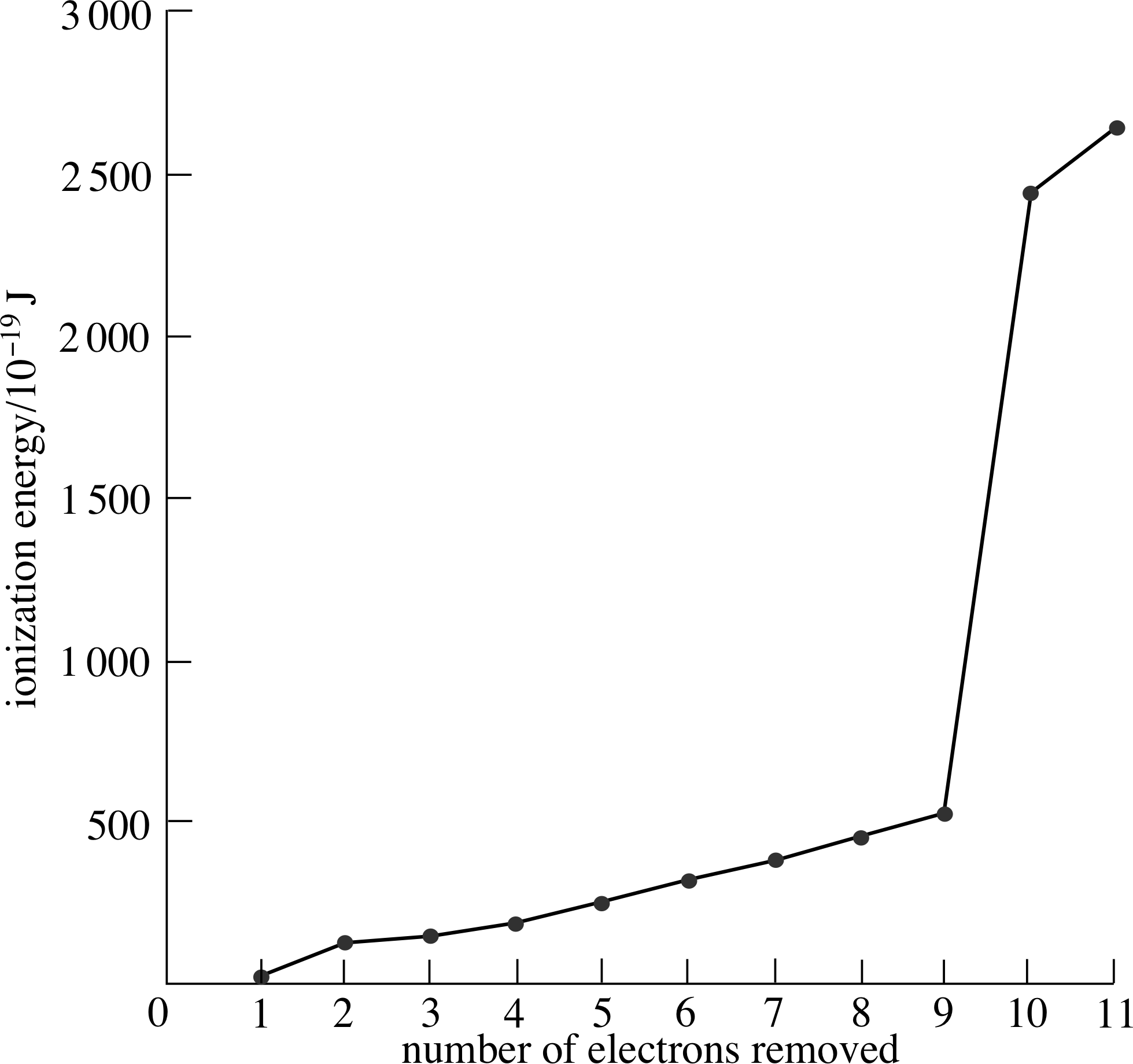
Figure 2 Successive ionization energies of sodium.
You might expect that the larger amounts of energy needed to remove successive electrons – the successive ionization energies – might perhaps increase in some uniform way. Figure 2 shows these energies for sodium. As you can see, each successive electron does require more energy to remove it, but successive ionization energies do not increase in a completely uniform way. The first electron is much more easily removed than subsequent ones and the energy needed to remove each of the next eight increases gradually but not quite uniformly. The last two electrons appear to be far more tightly bound to the atom since much larger amounts of energy are needed to free them.
It appears that the electrons in sodium fall into three groups. The first electron removed is in a different group from the next eight, and the last two electrons make the third group.
The fact that the pattern is obviously not uniform indicates that the successive ionization energies are influenced by some factor other than the regularly changing net charge of the atom (or ion).
✦ Treating each of the electrons and the nucleus as oppositely charged point particles, separated by some definite average distance, what does Coulomb’s law suggest about the average distance of the most loosely bound electrons from the atomic nucleus, compared with the average distances of the most tightly bound electrons?
✧ Coulomb’s law tells us that, for two oppositely charged point–like bodies, the greater the distance between them, the smaller the magnitude of the attractive electrostatic force between them. i) The law therefore suggests that the most loosely bound electron is relatively far from the nucleus, so this must be the atom’s outermost electron. The two most tightly bound electrons are relatively close to the nucleus, so these are the atom’s innermost electrons.
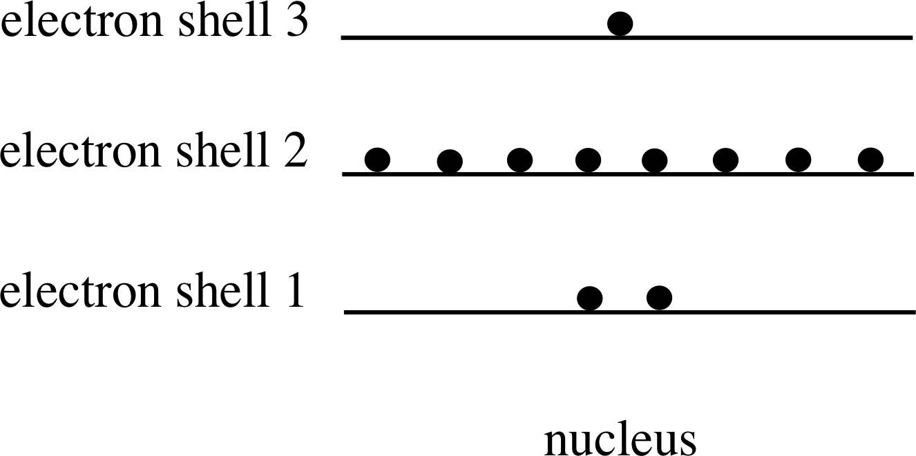
Figure 3 Electron shells for sodium.
As Figure 3 shows, we can imagine that the electrons (represented by spots) are in groups at various distances from a central nucleus, and that all the electrons within a given group have similar energies. In Figure 3 the similar energies of all members of a group are represented by just one energy. These groups are called electron shells. Following a well established convention, Figure 3 shows the electrons with the highest successive ionization energy (the most tightly bound) at the bottom of the figure.
The shells are numbered 1, 2, 3, etc., beginning with the most strongly bound state (i.e. the lowest energy level). The shell number is called the principal quantum number and is given the symbol n. This is one of four quantum numbers that, as you will discover in this module, are needed to specify completely the behaviour of an atomic electron. Figure 3 also suggests that electron shells have a limited capacity, since electrons might be expected to occupy the lowest possible energy level available, and so would only move into the n = 3 shell if the n = 1 and n = 2 shells had reached their capacity.
2.2 Photoelectron spectroscopy
Experiments on the successive ionization energies of all the chemical elements reveal that their electron shell structures are generalizations of that of sodium. For example, the first (n = 1) shell of each element is found to accommodate at most two electrons whereas the second (n = 2) shell can contain at most eight. In this way, the successive ionization energies provide a simple, though rather crude, picture of the energy levels of electrons in atoms.
This is about as far as we can go in developing the shell model of electron distributions in ground state atoms on the basis of successive ionization energies. The method faces a fundamental problem: as the original ground state atom is successively ionized the increasing net charge of the ion that results from each successive step will influence the energy levels of the remaining electrons. Hence, no matter how accurately we measure the successive ionization energies they do not readily yield accurate information about the shell structure of the ground state neutral atom. (In case you’ve forgotten, it was the distribution of electrons in the ground state atom that we set out to investigate.)
Fortunately, we can use the results of another investigative technique – photoelectron spectroscopy – to give direct information about energy levels in neutral (un-ionized) atoms. In this technique we can measure the energy required to remove each electron from the same uncharged atom rather than the energy to eject successive electrons from the increasingly charged ion. Let us now consider such experiments and the information they can yield.
When an atom absorbs a photon (i.e. a quantum of electromagnetic radiation) that has an energy higher than the atom’s ionization energy, the atom becomes ionized and an electron, referred to as a photoelectron in this context, is ejected from the atom. The principle of conservation of energy implies that the kinetic energy Ek of the photoelectron is equal to the difference between the photon energy and the threshold energy I i that is required to just remove that particular electron from the atom. The photon energy is given by Planck–Einstein formula as E = hf, where h is Planck’s constant (which is equal to 6.63 × 10⁻³⁴ J s) and f is the frequency of the electromagnetic radiation, so the kinetic energy Ek of the photoelectron is given by:
Ek = hf − I(1) i
This equation makes good intuitive sense: if the energy hf of the photon is less than I, the atomic electron will not be dislodged, whereas if the photon energy is greater than I, the electron will be ejected, and the greater the photon energy, the greater will be the kinetic energy of the electron. The equation also shows that if we know the photon energy, and if we can measure the kinetic energy of the electrons, we can determine the threshold energy I for the particular electron that was ejected. This identifies the binding energy of the shell or subshell from which the electron came.
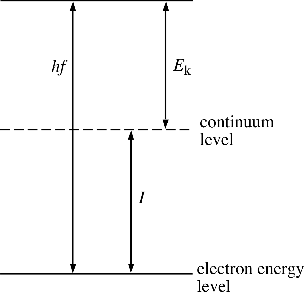
Figure 4 The relationship between the threshold energy I, the kinetic energy Ek of an ejected electron, and the photon energy hf.
The relationship between the terms in Equation 1 is more apparent if it is represented diagrammatically. Figure 4 shows the threshold energy as the difference in energy between the electron energy level and the continuum level (or ionization level) which represents the lowest energy that the electron must reach if it is to escape entirely from the atom.
This relationship between the threshold energy and the kinetic energy of the outgoing photoelectron is the basis of photoelectron spectroscopy. Two key features explain why photoelectron spectroscopy is a more powerful diagnostic technique than simple successive ionization. First, when a gas of neutral atoms is irradiated by electromagnetic radiation of sufficiently short wavelength, the photoionization usually removes one electron at a time, but it can be any one of the bound electrons in the atom which is removed. The outgoing photoelectron carries away kinetic energy which depends on the energy level from which it was removed.
In contrast, with ionization via an electron beam, such as in successive ionization, the least tightly bound electron must be removed before any more tightly bound electrons can go. The information on the deep levels within the neutral atom is thus not available from successive ionization studies. A second reason for the pre–eminence of photoelectron spectroscopy is the precision available. The wavelength of the incident radiation can be selected to very high precision via a spectrometer or a similar device and so the frequencies, and hence the photon energies, are also very well known. In contrast, the incident energy of an electron in an electron beam is much less well known. Photoelectron spectroscopy thus forms a much more precise diagnostic tool with which to study the deep levels within a neutral atom.
Electromagnetic radiation selected with a single frequency is known as monochromatic radiation. If the frequency of this type of radiation is known, the photon energy hf is also known and all that remains is to determine the kinetic energy of the photoelectrons that are ejected from the atoms. The threshold energy I of each ejected electron is then given by I = hf − Ek. The number of photoelectrons ejected with kinetic energy Ek is measured and interpreted as the number of ejected electrons with threshold energy I = hf − Ek. A plot of the number of photoelectrons detected against the threshold energy I is called a photoelectron spectrum.
Photoelectron spectra allow the energy levels of electrons in atoms to be examined directly, since each peak in a photoelectron spectrum corresponds to the threshold energy of an electron from a particular energy level of the neutral atom.
Figure 5 shows the simple relationship between the photoelectron spectrum of an atom with three occupied electron energy levels and the electron energy level diagram for that atom. Notice that when the spectrum is rotated clockwise through 90° it gives a picture of the occupied part of the electron energy level diagram. Notice too that the most tightly bound electrons (those with the highest threshold energies) occupy the lowest energy levels in the atom, and that the energy zero has been placed at the continuum level.
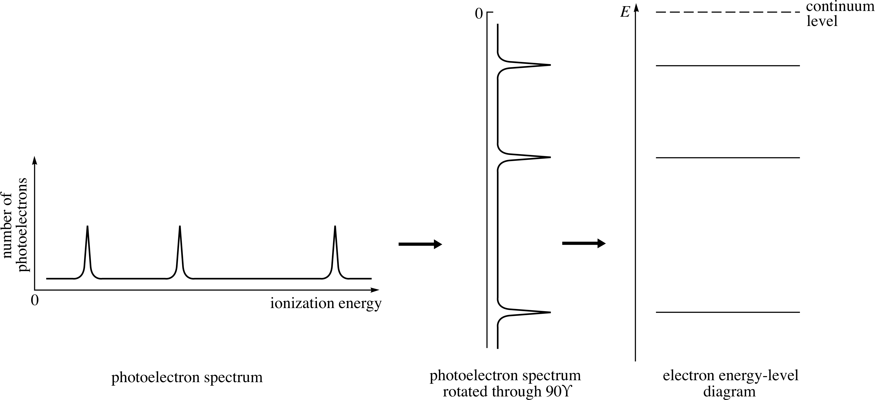
Figure 5 The relationship of the electron energy level diagram to the photoelectron spectrum. The presence of a peak in the photoelectron spectrum indicates the presence in the atom of electrons with the corresponding threshold energy.
Placing the energy zero at the continuum level may seem rather strange at first sight since it forces the energy levels of all the bound electrons to be negative, with the lowest energy level being the most negative. This choice of energy zero can be justified in general terms by saying that when the electron is far removed from the atom it is no longer interacting with the atom and so it is sensible to say that its potential energy is zero. If the electron is also at rest then the kinetic energy is also zero and so the total energy zero is sensibly chosen to be with the electron at rest and far removed from the atom. This is the continuum level and the choice of energy zero at the continuum level is also adopted in most situations in spectroscopy.
The photoelectron spectra of three gases, helium, neon and krypton are shown schematically in Figure 6. i In these spectra, the peaks are shown to have equal heights. In fact the heights of the peaks in a spectrum will not be exactly the same, because they depend on the number of electrons of a particular energy and on the likelihood of their photoemission. The ejection of the tightly bound electrons from atoms such as neon and krypton, requires very high energy photons, so X–rays are used. i
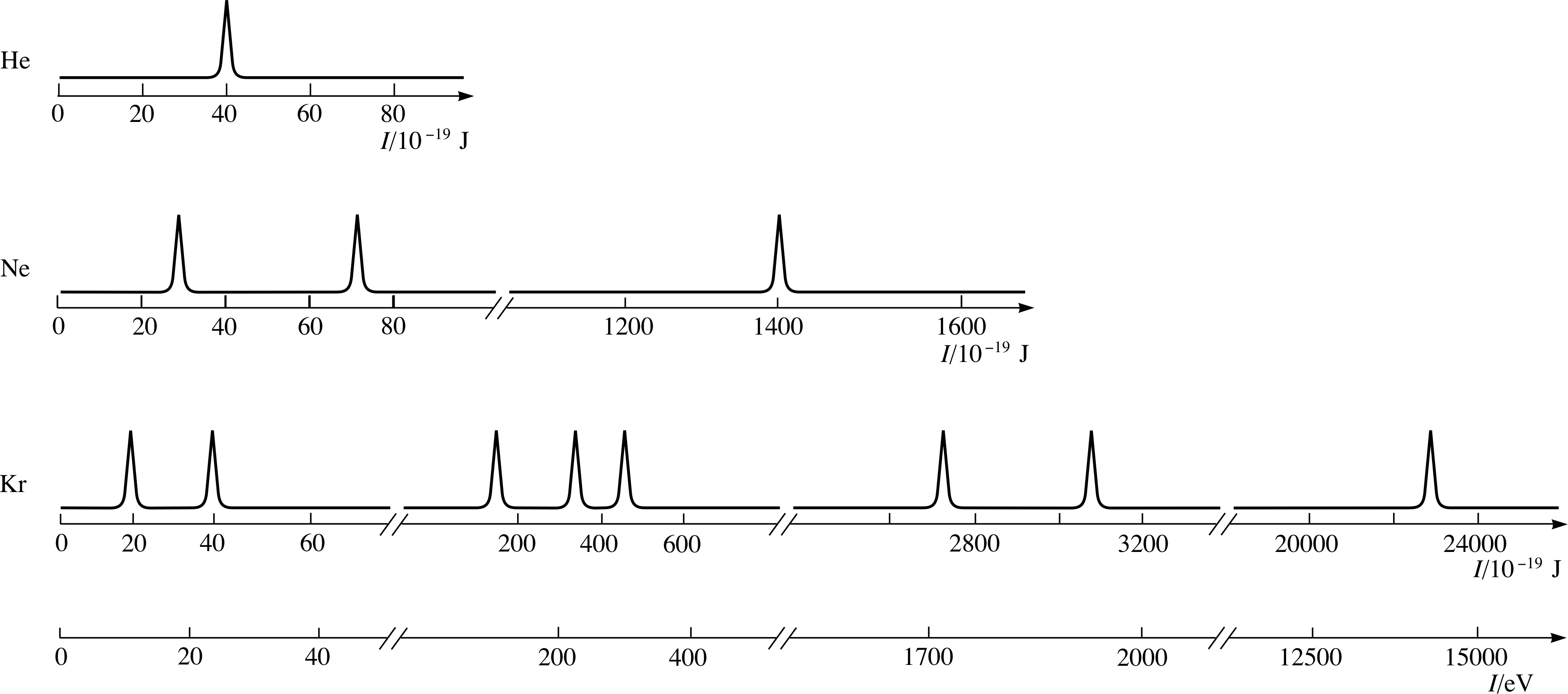
Figure 6 Schematic photoelectron spectra of helium, neon and krypton. Notice how the energy scales are broken and that large energy gaps occur between the groups of peaks.
The energy scale for the krypton spectrum in Figure 6 is graduated E using the joule, the familiar SI unit of energy, and also using the electronvolt (eV), which is defined to be the kinetic energy gained by an electron that has been accelerated through a potential difference of one volt (1 eV ≈ 1.6 × 10⁻¹⁹ J). This comparatively tiny unit of energy is much more convenient than the joule when dealing with atomic physics.
To interpret photoelectron spectra you need to know how many electrons are contained in each type of neutral atom (this is given by the atomic number Z of the relevant chemical element). In the case of helium, for which Z = 2, there are two electrons in the neutral atom, so the presence of a single peak in the helium photoelectron spectrum implies that both electrons occupy the same energy level in the atom.
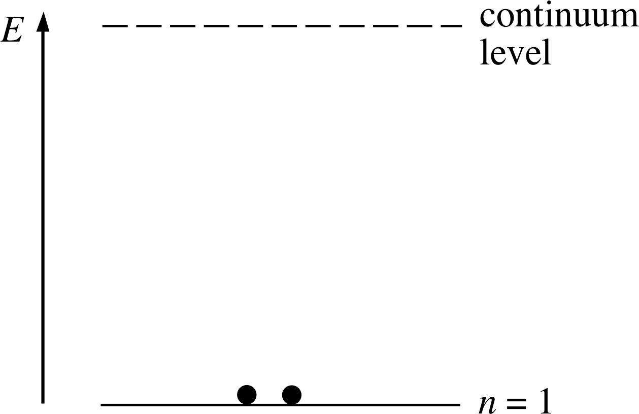
Figure 7 The electron energy level diagram of a helium atom in its ground state.
This is represented diagrammatically in Figure 7. Notice that the occupied electron energy level is labelled n = 1.
Three notable features of the spectra in Figure 6 are:
- 1
-
The spectra of neon and krypton contain more than one peak.
- 2
-
The number of peaks for these three gases increases with atomic number.
- 3
-
Within a spectrum the peaks fall into groups, each of which spans a relatively small range in the values of I. For example there are three peaks in the krypton spectrum in the range 150 × 10−19 J to 450 × 10−19 J.
On the other hand, the energy differences between groups are considerably larger than the width of each group.
2.3 Interpretation in terms of shells and subshells
In this subsection, we shall argue that the principal quantum number n is insufficient, by itself, to specify fully the state of an atomic electron. This will lead us to introduce the second of the four quantum numbers that are actually required.
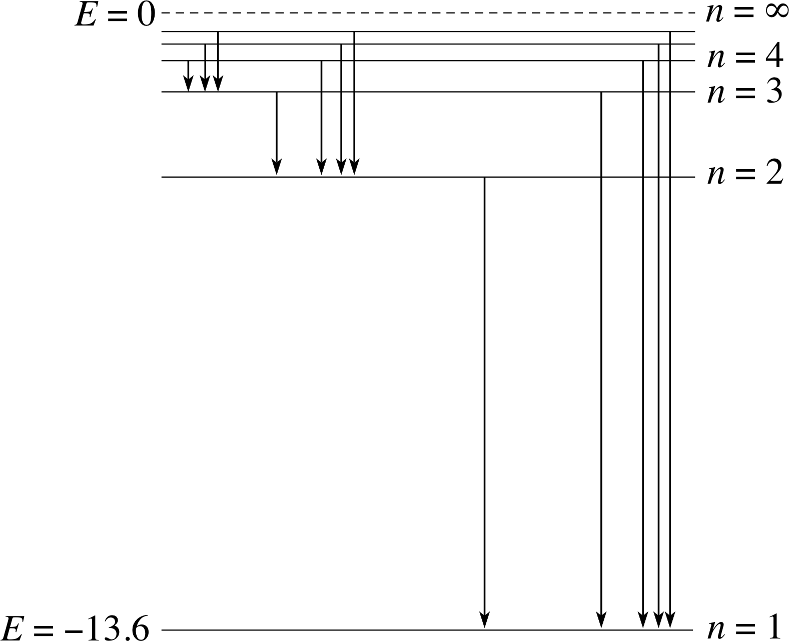
Figure 8 The energy levels of the hydrogen atom. When the hydrogen atom is in its ground state, only the lowest lying n = 1 level is occupied. Note that E is measured in eV.
The relationship between the photoelectron spectra in Figure 6 and the corresponding diagrams of (occupied) energy levels is easily seen. As in Figure 5, you have to imagine turning the spectra through 90° so that they are arranged vertically with I = 0 (which corresponds to the continuum level) at the top. Viewing the spectra in this way it is quite clear that the occupied energy levels of neon (Figure 6) form two groups (a single level of 1400 × 10−19 J and a pair of levels on either side of 50 × 10−19 J ), while the occupied levels of krypton form four groups. It is instructive to compare these groups of occupied levels with the energy levels of atomic hydrogen, the lowest of which are shown in Figure 8.
The comparison between Figure 8, for hydrogen, and, for example, Figure 3 for sodium is a matter of frequent confusion.
Figure 3 Electron shells for sodium.
Hydrogen has a single electron and if we were to construct its ground state diagram along the lines of Figure 3 then there would be a single electron shell n = 1 with a single electron in this shell. The shells at n = 2 and n = 3 would be empty. If this ground state atom is then given more energy so that its single electron could reach the n = 2, n = 3... shells, then we obtain the additional excited energy levels shown in Figure 8, and the consequent emission spectral lines via transition to lower energy levels.
In contrast, Figure 3 for the sodium atom shows the ground state of the atom, with the n =1 and n=2 shells already filled and with the final electron in the n = 3 shell, but with no possibility of it making a transition to n = 2 or n = 1, since there is no vacancy in these shells. We could add energy to the ground state sodium atom to produce electrons in its excited levels above n = 3 or into levels within other subshells of n = 3.
As you can see, in the case of hydrogen each of the levels corresponds to a different value of the principal quantum number n, and the levels get closer together as n increases and the threshold energies to the ionization level from these shells decrease.
This is very similar to the behaviour of neon and krypton, where the groups of energy levels (as well as the levels themselves) get closer together as the threshold energy decreases. This suggests that in the case of such multi–electron atoms each group of energy levels corresponds to a single value of the principal quantum number, and that within each group some other quantum number is required to distinguish one energy level from another. This same point is clear from Figure 6. For example, in the case of neon there are eight electrons in the n = 2 shell but they have two different threshold energies. Six electrons are bound rather less strongly than the other two electrons. It follows that a second label is required to distinguish these two groups and so we need a second quantum number, in addition to the shell quantum number n. We shall denote this new quantum number by l and for the moment we shall just refer to it as the second quantum number; its physical significance will be explained in Section 4.
A final point in the comparison between hydrogen and other atoms may be worrying you. It is simply the question why, in Figure 8 for hydrogen, we do not need to draw separate energy levels for the subshells, as we do for other atoms. For hydrogen the excited energy levels are labelled by their shell number n, without any regard for the possible l values within each of these shells. The reason for this is that although such possibilities also exist for hydrogen, the electron energy for hydrogen does not depend on the subshell label l. Hydrogen is unique in that the energy of the electron is independent of the l value! The explanation of this exceptional behaviour of hydrogen lies in its structure. i
✦ Can you think of a way in which the structure of hydrogen is different from all other atoms?
✧ Hydrogen is the only atom which has a single electron – all other atoms have several electrons. It turns out that it is the interaction between electrons in an atom (rather than that between electrons and the nucleus) which causes the energy dependence on l. This is why hydrogen is different from all other atoms in this respect – the full story behind this lies beyond FLAP but you should appreciate the basic point here.
In keeping with our use of the term shell when describing the pattern of successive ionization energies in Subsection 2.1, we may now say that each value of n corresponds to a particular electron shell, and that for a given value of n each value of l corresponds to a different subshell.
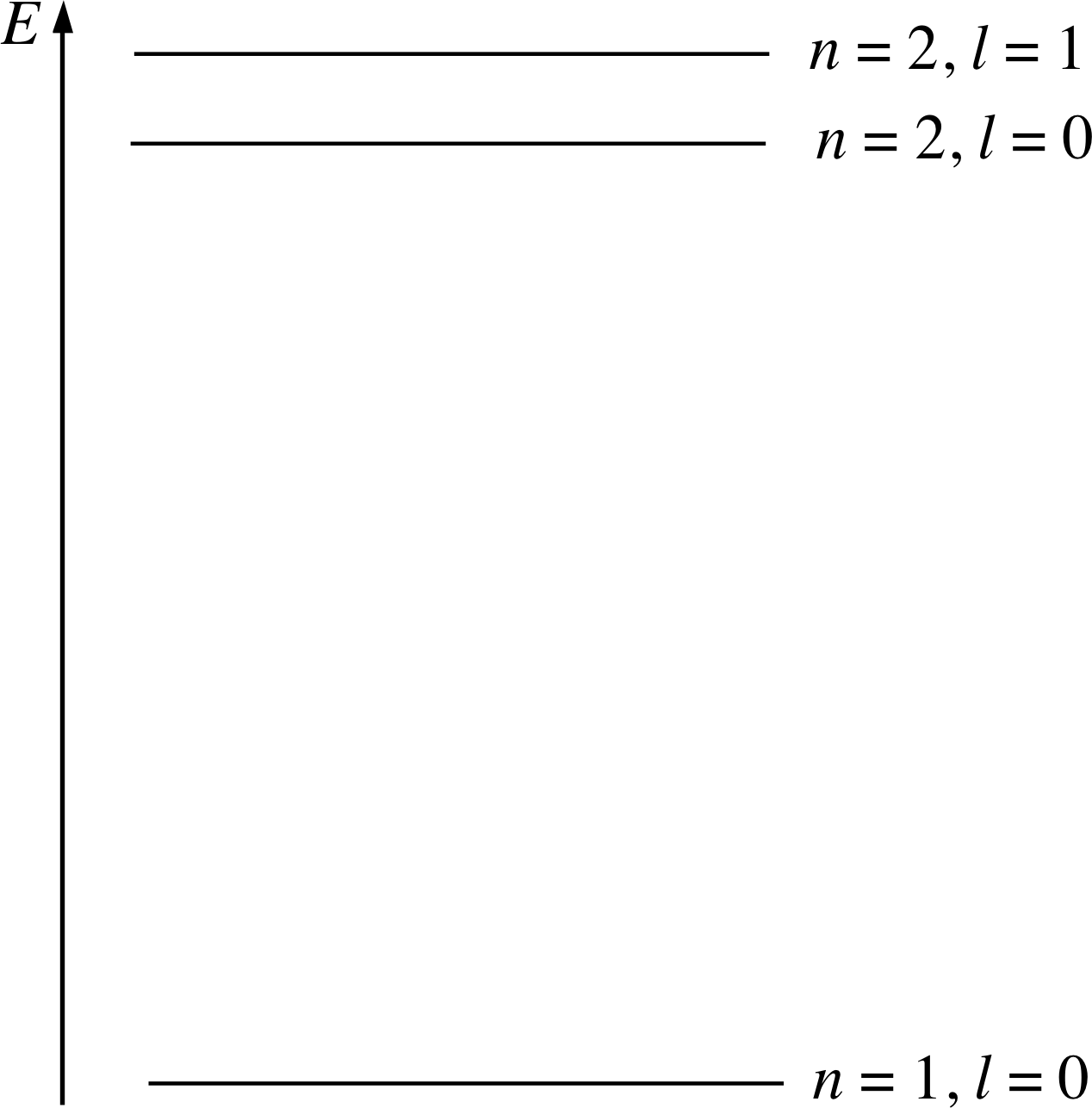
Figure 10 The occupied energy levels of the ground state neon atom, labelled with the appropriate values of n and l. (Not to scale)
For reasons that will become clear later, l is chosen so that it has only positive integer values starting with 0. Thus, in the case of neon for example, we can interpret the spectrum of Figure 6 as showing the presence of two shells (n = 1 and n = 2) with the n = 2 shell divided into two subshells with l = 0 and l = 1; this interpretation is shown in Figure 9.
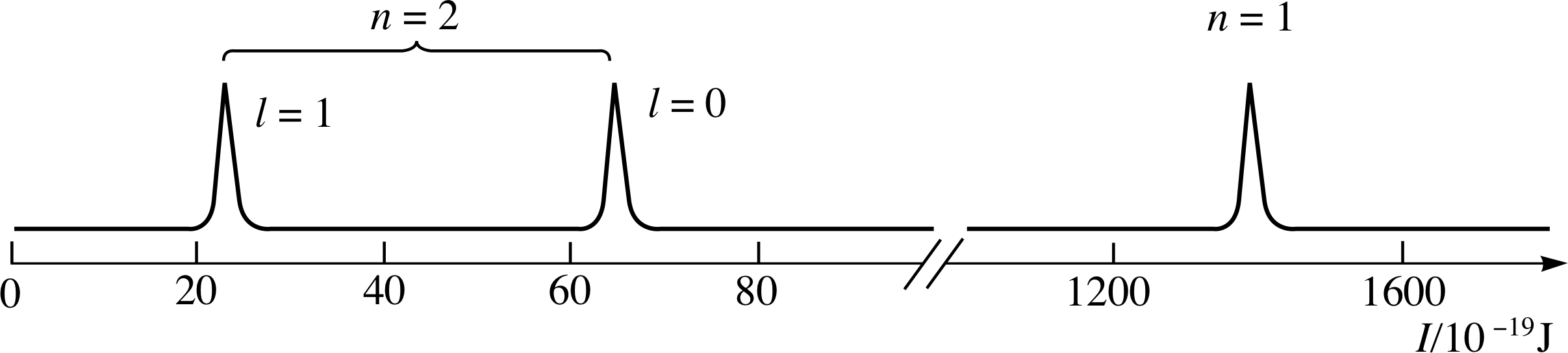
Figure 9 A schematic photoelectron spectrum for neon interpreted in terms of the quantum numbers n and l.
The corresponding energy level diagram is shown in Figure 10. (Note that by assigning l = 0 to the subshell with the higher threshold energy we ensure that it will be the lower of the n = 2 energy levels.)
Question T1
Draw an energy level diagram for krypton, based on its photoelectron spectrum (Figure 6) and label it with the appropriate values of n and l.
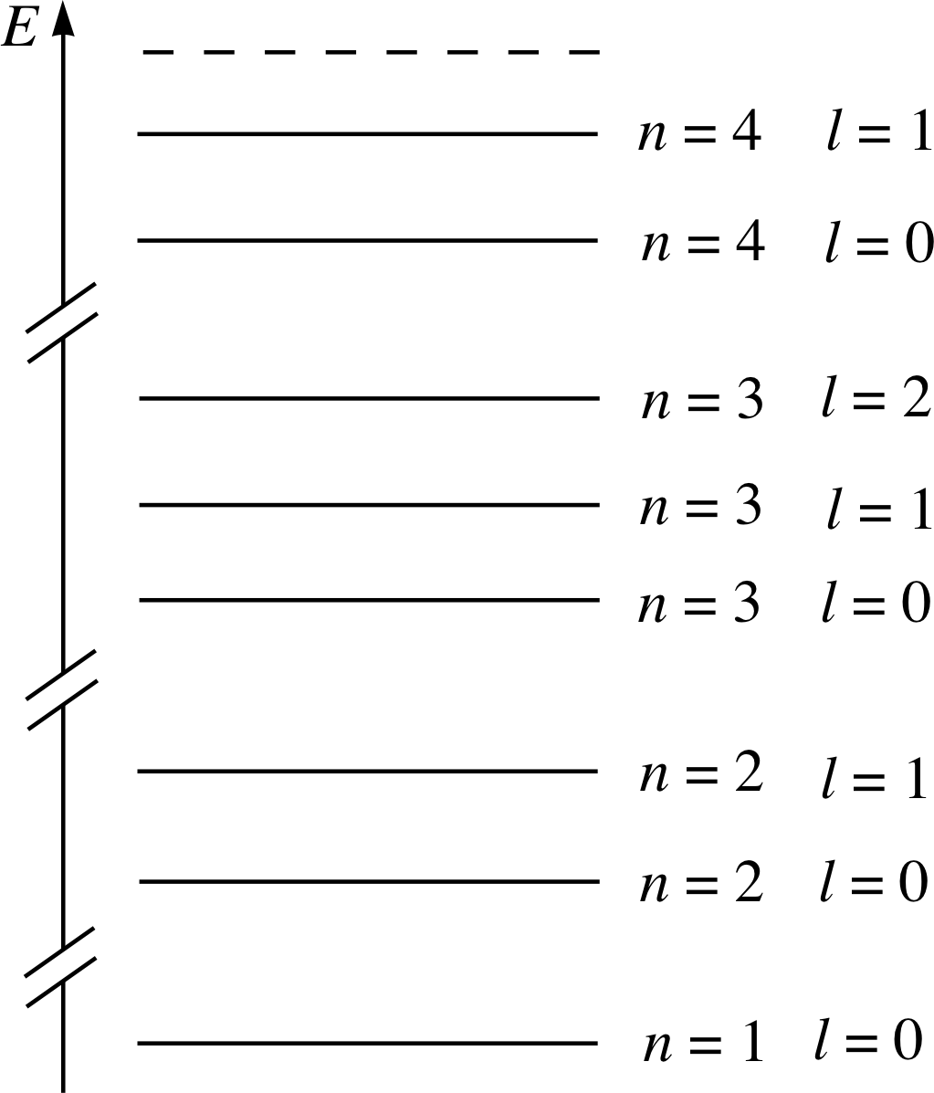
Figure 24 See Answer T1.
Answer T1
The labels on your diagram should be the same as the values of n shown in the energy level diagram for krypton in Figure 24. The lowest energy level corresponds to the highest energy peak on the right of the photoelectron spectrum.
Your diagram of the occupied energy levels of krypton should indicate an important feature of the general relationship between the shells and subshells of multi–electron atoms. This feature is the subject of the next question.
✦ In the case of krypton, how many subshells are there in each of the shells n = 1, n = 2 and n = 3?
✧ The n = 1 shell has one subshell (l = 0).
The n = 2 shell has two subshells (l = 0 and l = 1).
The n = 3 shell has three subshells (l = 0, l = 1 and l = 2).
These particular observations are indicative of the general result that a shell with principal quantum number n always contains n subshells which may be labelled by integer values of l from l = 0 to l = n − 1.
The existence of this general relationship between the principal quantum number of a shell and the number of subshells that it contains raises another question about the results we have already quoted.
✦ Why does the ground state photoelectron spectrum of krypton (in Figure 6) provide evidence of only two subshells in the n = 4 shell, where four might be expected?
✧ The photoelectron spectrum of ground state krypton atoms will only provide evidence of those energy levels that are occupied in the ground state. There are four subshells corresponding to n = 4, but only two are occupied when the atom is in its ground state, so they are the only ones that are observed. There are simply not enough electrons to occupy the other subshells in krypton.
We can summarize our findings regarding energy levels as follows:
The energy levels of an atom may be divided into groups called shells, which may be further subdivided into subshells. Each shell corresponds to a particular value of the principal quantum number n (n = 1, 2, 3, ... etc.). Within a shell with principal quantum number n, there are n subshells, each of which corresponds to a particular value of a second quantum number l (l = 0, 1, 2, 3, ... n − 1).
Apart from the lightest elements, hydrogen and helium, every element has an atomic ground state that involves more than one occupied shell. Moreover, the number of occupied shells tends to increase with the atomic number of the element (and hence with the number of electrons in each atom). The most plausible explanation of this observation, as we pointed out in Subsection 2.1, is that there is a limit to the number of electrons that can occupy any given level. Thus, in the ground state, the lowest lying energy level of an atom will be the first to be occupied but when it has accommodated as many electrons as possible the next lowest energy level will start to fill, and so on, until all the electrons have been accommodated.
Given that this is broadly the case, it is clear that in order to predict the ground state of any atom we need to know the maximum number of electrons that can occupy each of the shells and subshells of that atom. This is the subject of the next section.
Question T2
Considering electrons in the n = 3 shell of krypton, which would you expect to be the most tightly bound to the atom, those in the l = 0 subshell or those in the l = 2 subshell?
Answer T2
The most tightly bound electrons will be those in the l = 0 subshell since they will have the higher threshold energy I.
3 Capacities of shells and subshells
3.1 Empirical rules for the capacities of shells and subshells
Experimental investigations of atoms based on photoelectron spectroscopy and more traditional techniques, such as conventional atomic spectroscopy, can be used to deduce empirical rules for the maximum number of electrons that may occupy any given shell or subshell. We could simply quote these rules at this point but rather than doing so we will first try to make them plausible by assuming that some of the results we have already discussed apply to atoms in general and not just to the particular cases we have investigated. From a logical point of view this is generally a dangerous thing to do, but in this case we are willing to take the risk because our conclusions are supported by many other experiments and may be given a firm theoretical foundation.
Figure 3 Electron shells for sodium.
If you look back to Figure 3, which was based on the successive ionization energies of sodium, you will see there are two electrons in the n = 1 shell and eight electrons in the n = 2 shell. There is also an electron in the n = 3 shell, so it seems likely that both the lower shells are full. Since the single occupied shell in helium (n = 1, l = 0) also accommodates two electrons, it seems reasonable to suppose that:
The n = 1, l = 0 subshell in all atoms holds a maximum of two electrons.
In fact, experiments indicate an even more general rule along these lines:
The maximum number of electrons that can occupy a subshell corresponding to a given value of l is entirely determined by the value of l, and does not depend on the value of n at all.
Combining these two rules leads to the following conclusion:
All subshells with l = 0 can accommodate a maximum of two electrons.
Using the information you already possess concerning the sodium atom, you should be able to use these rules to discover the maximum number of electrons that can be accommodated in any l = 1 subshell.
Question T3
| Shell | Subshell | Maximum no. of electrons in the subshell |
|---|---|---|
| n = 1 | l = 0 | |
| n = 2 | l = 0 | |
| n = 2 | l = 1 |
Complete Table 1 by entering the maximum number of electrons in each of the subshells in the first two electron shells.
| Shell | Subshell | Maximum no. of electrons in the subshell |
|---|---|---|
| n = 1 | l = 0 | 2 |
| n = 2 | l = 0 | 2 |
| n = 2 | l = 1 | 6 |
Answer T3
The missing numbers are from the top: two, two and six.
Figure 10 The occupied energy levels of the ground state neon atom, labelled with the appropriate values of n and l. (Not to scale)
Figure 7 The electron energy level diagram of a helium atom in its ground state.
Question T4
Complete Figure 10 by drawing in the dots to represent electrons in neon, in the same way as in Figure 7. The atomic number of neon is Z = 10, so an atom of neon contains ten electrons.
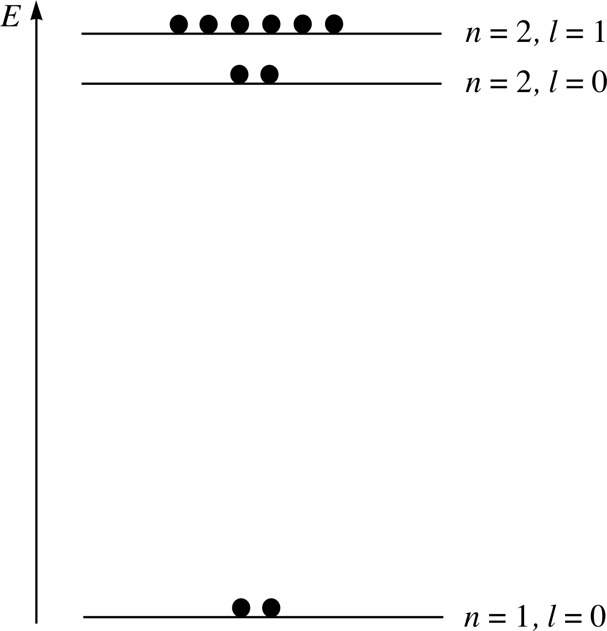
Figure 25 See Answer T4.
Answer T4
Your completed diagram for neon should look like Figure 25 which gives the occupation of energy levels in the neon atom.
Further information about the numbers of electrons in subshells can be obtained by examining heavier atoms. For example, consider the photoelectron spectrum of krypton in Figure 6. The atomic number of krypton is 36, and the atom contains electrons in the n = 1, n = 2, n = 3 and n = 4 shells; this indicates that the n = 3, l = 2 subshell is probably full in this particular atom.
How can we find out how many electrons are in the n = 3, l = 2 subshell of krypton?
First we need to know the total number in the n = 3 shell. We can determine this by subtracting the total number in all the other shells from the krypton atom’s full complement of 36 electrons. We know there will be two electrons in a full n = 1 shell and eight in a full n = 2 shell, but the n = 4 shell is more of a problem since we don’t know how many electrons it might contain. Fortunately only two of the n = 4 subshells are occupied, presumably l = 0 and l = 1, and we know that their combined capacity is eight electrons, but we still can’t be sure that they are full. However, the photoelectron spectrum of the element rubidium (which has one more electron per atom than krypton) contains an additional peak, which indicates that the n = 4, l = 0 and n = 4, l = 1 subshells of krypton probably are full. Making this assumption it follows that there are eight electrons in the occupied part of the n = 4 shell, and that the number of electrons in the full n = 3 shell is 36 − 18 = 18.
Question T5
How many electrons fill the n = 3, l = 2 subshell of krypton, and by implication how many electrons fill any l = 2 subshell?
Answer T5
Since the full n = 3 shell contains 18 electrons and we already know there are two in the l = 0 subshell and six in the l = 1 subshell, it follows that ten electrons are needed to fill the l = 2 subshell.
Since these capacities are always general results, it follows that ten is the maximum capacity of any l = 2 subshell.
Similar aguments involving even heavier atoms lead to the conclusion that
All subshells with l = 3 can accommodate a maximum of fourteen electrons.
Knowing the capacity of the subshells corresponding to l = 0, 1, 2 and 3, and remembering that shell n contains subshells with l = 0, 1, ... n − 1, it is a simple matter to determine the total capacity of the first few shells. You can confirm for yourself that the results are as follows:
- 2 electrons fill n =1
- 8 electrons fill n = 2
- 18 electrons fill n = 3
- 32 electrons fill n = 4
Obviously, we could continue this process if we knew the capacity of subshells with l = 4.
The various empirical results for the capacities of shells and subshells that we have obtained in this subsection may be summarized by a pair of remarkably simple rules that turn out to be generally true in the sense that they hold true for all allowed values of n and l. These rules are as follows:
The maximum number of electrons that can occupy a subshell with second quantum number l is 2(2l + 1).
The maximum number of electrons that can occupy a shell with principal quantum number n is 2n2.
The second of these rules is a consequence of the first and the fact that in the nth shell l = 0, 1, 2, ... n − 1. i But the origin of the first rule and the reason for the restriction on the values of l is not at all clear at this stage. We shall return to these puzzles in Section 4.
3.2 s-p-d-f notation
The energy levels of atoms were originally established by conventional atomic spectroscopy, i.e. by observing the light emitted by excited atoms. In many atoms the lines seen in these emission spectra form a number of overlapping series_spectroscopicseries. For example, in sodium one of these consists of sharp lines and another of diffuse lines, while a third series is known as the principal series because it is the most intense. As atomic physics developed, these series came to be connected with particular values of the second quantum number of the upper level for the transition. For that reason the value of the second quantum number is often indicated by the initial letters of the associated series, s, p, d and f (f comes from fundamental), so instead of using numbers for particular values of l, we may write:
- s for subshells with l = 0
- p for subshells with l = 1
- d for subshells with l = 2
- f for subshells with l = 3
This s–p–d–f notation is very commonly used as a shorthand method of labelling electron energy levels.
For example, if the lowest energy level in an atom has n = 1 and l = 0, it is said to be a 1s level.
✦ What is the shorthand notation for the atomic energy level that corresponds to n = 4 and l = 3?
✧ 4f
(remember l = 3 subshells are labelled f).
Figure 10 The occupied energy levels of the ground state neon atom, labelled with the appropriate values of n and l. (Not to scale)
Question T6
Label the levels in Figure 10 using the s-p-d-f notation.
Answer T6
From the bottom up, the levels should be labelled 1s, 2s, 2p.
3.3 Ground state electronic configurations of the elements
We now have almost enough information to start predicting the distribution of electrons in the shells and subshells of any atom in its ground state (i.e. its lowest energy state). This distribution is called the element’s ground state electronic configuration.
The s-p-d-f notation may be used to indicate how the electrons of a given atom are distributed amongst the various energy levels. For example, an atom of helium in its ground state has two electrons in the 1s level, we therefore say that it has ‘two 1s electrons’ and we write that number of electrons as a superscript after the letter s. The electronic configuration of helium is therefore written as 1s2 which may be read as ‘one s two’.
A lithium atom in its ground state has an additional electron in the 2s subshell, so its ground state may be written 1s2 2s. i The electronic configurations of the ground states of other atoms can also be written in this way.
Figure 10 The occupied energy levels of the ground state neon atom, labelled with the appropriate values of n and l. (Not to scale)
✦ Taking account of the information in your completed Figure 10, write the electronic configuration of the ground state of a neon atom using the s-p-d-f notation.
✧ The ground state electronic configuration of neon is 1s2 2s2 2p6.
Question T7
Figure 11 shows the electron energy level diagrams for several elements, with the electrons (each depicted here as a black dot) already inserted in the diagram for sodium (Z = 11). Complete the diagrams for beryllium, argon and bromine in a similar way, given that their atomic numbers are 4, 18 and 35, respectively.

Figure 11 Schematic energy level diagrams for the ground states of atoms of four chemical elements – sodium,
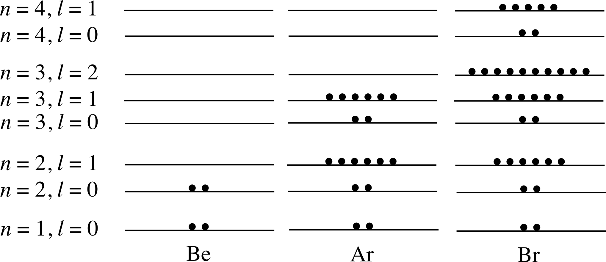
Figure 26 See Answer T7.
Answer T7
Your diagrams for Be, Ar and Br should resemble those in Figure 26.
✦ What is the ground state electronic configuration of sodium?
✧ The ground state configuration of sodium is 1s2 2s2 2p6 3s.
You might think that you could now continue this process, using the known capacities of the various shells and subshells, to draw the energy level diagram and determine the ground state electronic configurations of all the elements. However, things are not quite that simple.
Our notation so far is little more than a classification system for electrons in a complex atom. We are still very far from being able to calculate these energy levels. For example, we expect energy to increase along the sequence 3s, 3p, 3d, 4s..., but we have not justified this at all! It seems likely but that is very different from a rigorous justification.
Table 2 shows the ground state electronic configurations of the elements.
| Z | 1s | 2s | 2p | 3s | 3p | 3d | 4s | 4p | 4d | 4f | 5s | 5p | 5d | 5f | 6s | 6p | 6d | 7s | |
|---|---|---|---|---|---|---|---|---|---|---|---|---|---|---|---|---|---|---|---|
| 1 | H | 1 | |||||||||||||||||
| 2 | He | 2 | |||||||||||||||||
| 3 | Li | 2 | 1 | ||||||||||||||||
| 4 | Be | 2 | 2 | ||||||||||||||||
| 5 | B | 2 | 2 | 1 | |||||||||||||||
| 6 | C | 2 | 2 | 2 | |||||||||||||||
| 7 | N | 2 | 2 | 3 | |||||||||||||||
| 8 | O | 2 | 2 | 4 | |||||||||||||||
| 9 | F | 2 | 2 | 5 | |||||||||||||||
| 10 | Ne | 2 | 2 | 6 |
| Z | 1s | 2s | 2p | 3s | 3p | 3d | 4s | 4p | 4d | 4f | 5s | 5p | 5d | 5f | 6s | 6p | 6d | 7s | |
|---|---|---|---|---|---|---|---|---|---|---|---|---|---|---|---|---|---|---|---|
| 11 | Na | 2 | 2 | 6 | 1 | ||||||||||||||
| 12 | Mg | 2 | 2 | 6 | 2 | ||||||||||||||
| 13 | Al | 2 | 2 | 6 | 2 | 1 | |||||||||||||
| 14 | Si | 2 | 2 | 6 | 2 | 2 | |||||||||||||
| 15 | P | 2 | 2 | 6 | 2 | 3 | |||||||||||||
| 16 | S | 2 | 2 | 6 | 2 | 4 | |||||||||||||
| 17 | Cl | 2 | 2 | 6 | 2 | 5 | |||||||||||||
| 18 | Ar | 2 | 2 | 6 | 2 | 6 | |||||||||||||
| 19 | K | 2 | 2 | 6 | 2 | 6 | 1 | ||||||||||||
| 20 | Ca | 2 | 2 | 6 | 2 | 6 | 2 |
| Z | 1s | 2s | 2p | 3s | 3p | 3d | 4s | 4p | 4d | 4f | 5s | 5p | 5d | 5f | 6s | 6p | 6d | 7s | |
|---|---|---|---|---|---|---|---|---|---|---|---|---|---|---|---|---|---|---|---|
| 21 | Sc | 2 | 2 | 6 | 2 | 6 | 1 | 2 | |||||||||||
| 22 | Ti | 2 | 2 | 6 | 2 | 6 | 2 | 2 | |||||||||||
| 23 | V | 2 | 2 | 6 | 2 | 6 | 3 | 2 | |||||||||||
| 24 | Cr | 2 | 2 | 6 | 2 | 6 | 5 | 1 | |||||||||||
| 25 | Mn | 2 | 2 | 6 | 2 | 6 | 5 | 2 | |||||||||||
| 26 | Fe | 2 | 2 | 6 | 2 | 6 | 6 | 2 | |||||||||||
| 27 | Co | 2 | 2 | 6 | 2 | 6 | 7 | 2 | |||||||||||
| 28 | Ni | 2 | 2 | 6 | 2 | 6 | 8 | 2 | |||||||||||
| 29 | Cu | 2 | 2 | 6 | 2 | 6 | 10 | 1 | |||||||||||
| 30 | Zn | 2 | 2 | 6 | 2 | 6 | 10 | 2 |
| Z | 1s | 2s | 2p | 3s | 3p | 3d | 4s | 4p | 4d | 4f | 5s | 5p | 5d | 5f | 6s | 6p | 6d | 7s | |
|---|---|---|---|---|---|---|---|---|---|---|---|---|---|---|---|---|---|---|---|
| 31 | Ga | 2 | 2 | 6 | 2 | 6 | 10 | 2 | 1 | ||||||||||
| 32 | Ge | 2 | 2 | 6 | 2 | 6 | 10 | 2 | 2 | ||||||||||
| 33 | As | 2 | 2 | 6 | 2 | 6 | 10 | 2 | 3 | ||||||||||
| 34 | Se | 2 | 2 | 6 | 2 | 6 | 10 | 2 | 4 | ||||||||||
| 35 | Br | 2 | 2 | 6 | 2 | 6 | 10 | 2 | 5 | ||||||||||
| 36 | Kr | 2 | 2 | 6 | 2 | 6 | 10 | 2 | 6 | ||||||||||
| 37 | Rb | 2 | 2 | 6 | 2 | 6 | 10 | 2 | 6 | 1 | |||||||||
| 38 | Sr | 2 | 2 | 6 | 2 | 6 | 10 | 2 | 6 | 2 |
| Z | 1s | 2s | 2p | 3s | 3p | 3d | 4s | 4p | 4d | 4f | 5s | 5p | 5d | 5f | 6s | 6p | 6d | 7s | |
|---|---|---|---|---|---|---|---|---|---|---|---|---|---|---|---|---|---|---|---|
| 39 | Y | 2 | 2 | 6 | 2 | 6 | 10 | 2 | 6 | 1 | 2 | ||||||||
| 40 | Zr | 2 | 2 | 6 | 2 | 6 | 10 | 2 | 6 | 2 | 2 | ||||||||
| 41 | Nb | 2 | 2 | 6 | 2 | 6 | 10 | 2 | 6 | 4 | 1 | ||||||||
| 42 | Mo | 2 | 2 | 6 | 2 | 6 | 10 | 2 | 6 | 5 | 1 | ||||||||
| 43 | Tc | 2 | 2 | 6 | 2 | 6 | 10 | 2 | 6 | 6 | 1 | ||||||||
| 44 | Ru | 2 | 2 | 6 | 2 | 6 | 10 | 2 | 6 | 7 | 1 | ||||||||
| 45 | Rh | 2 | 2 | 6 | 2 | 6 | 10 | 2 | 6 | 8 | 1 | ||||||||
| 46 | Pd | 2 | 2 | 6 | 2 | 6 | 10 | 2 | 6 | 10 | |||||||||
| 47 | Ag | 2 | 2 | 6 | 2 | 6 | 10 | 2 | 6 | 10 | 1 | ||||||||
| 48 | Cd | 2 | 2 | 6 | 2 | 6 | 10 | 2 | 6 | 10 | 2 |
| Z | 1s | 2s | 2p | 3s | 3p | 3d | 4s | 4p | 4d | 4f | 5s | 5p | 5d | 5f | 6s | 6p | 6d | 7s | |
|---|---|---|---|---|---|---|---|---|---|---|---|---|---|---|---|---|---|---|---|
| 49 | In | 2 | 2 | 6 | 2 | 6 | 10 | 2 | 6 | 10 | 2 | 1 | |||||||
| 50 | Sn | 2 | 2 | 6 | 2 | 6 | 10 | 2 | 6 | 10 | 2 | 2 | |||||||
| 51 | Sb | 2 | 2 | 6 | 2 | 6 | 10 | 2 | 6 | 10 | 2 | 3 | |||||||
| 52 | Te | 2 | 2 | 6 | 2 | 6 | 10 | 2 | 6 | 10 | 2 | 4 | |||||||
| 53 | I | 2 | 2 | 6 | 2 | 6 | 10 | 2 | 6 | 10 | 2 | 5 | |||||||
| 54 | Xe | 2 | 2 | 6 | 2 | 6 | 10 | 2 | 6 | 10 | 2 | 6 | |||||||
| 55 | Cs | 2 | 2 | 6 | 2 | 6 | 10 | 2 | 6 | 10 | 2 | 6 | 1 | ||||||
| 56 | Ba | 2 | 2 | 6 | 2 | 6 | 10 | 2 | 6 | 10 | 2 | 6 | 2 |
| Z | 1s | 2s | 2p | 3s | 3p | 3d | 4s | 4p | 4d | 4f | 5s | 5p | 5d | 5f | 6s | 6p | 6d | 7s | |
|---|---|---|---|---|---|---|---|---|---|---|---|---|---|---|---|---|---|---|---|
| 57 | La | 2 | 2 | 6 | 2 | 6 | 10 | 2 | 6 | 10 | 2 | 6 | 1 | 2 | |||||
| 58 | Ce | 2 | 2 | 6 | 2 | 6 | 10 | 2 | 6 | 10 | 2 | 2 | 6 | 2 | |||||
| 59 | Pr | 2 | 2 | 6 | 2 | 6 | 10 | 2 | 6 | 10 | 3 | 2 | 6 | 2 | |||||
| 60 | Nd | 2 | 2 | 6 | 2 | 6 | 10 | 2 | 6 | 10 | 4 | 2 | 6 | 2 | |||||
| 61 | Pm | 2 | 2 | 6 | 2 | 6 | 10 | 2 | 6 | 10 | 5 | 2 | 6 | 2 | |||||
| 62 | Sm | 2 | 2 | 6 | 2 | 6 | 10 | 2 | 6 | 10 | 6 | 2 | 6 | 2 | |||||
| 63 | Eu | 2 | 2 | 6 | 2 | 6 | 10 | 2 | 6 | 10 | 7 | 2 | 6 | 2 | |||||
| 64 | Gd | 2 | 2 | 6 | 2 | 6 | 10 | 2 | 6 | 10 | 7 | 2 | 6 | 1 | 2 | ||||
| 65 | Tb | 2 | 2 | 6 | 2 | 6 | 10 | 2 | 6 | 10 | 9 | 2 | 6 | 2 | |||||
| 66 | Dy | 2 | 2 | 6 | 2 | 6 | 10 | 2 | 6 | 10 | 10 | 2 | 6 | 2 | |||||
| 66 | Ho | 2 | 2 | 6 | 2 | 6 | 10 | 2 | 6 | 10 | 11 | 2 | 6 | 2 | |||||
| 68 | Er | 2 | 2 | 6 | 2 | 6 | 10 | 2 | 6 | 10 | 12 | 2 | 6 | 2 | |||||
| 69 | Tm | 2 | 2 | 6 | 2 | 6 | 10 | 2 | 6 | 10 | 13 | 2 | 6 | 2 | |||||
| 70 | Yb | 2 | 2 | 6 | 2 | 6 | 10 | 2 | 6 | 10 | 14 | 2 | 6 | 2 |
| Z | 1s | 2s | 2p | 3s | 3p | 3d | 4s | 4p | 4d | 4f | 5s | 5p | 5d | 5f | 6s | 6p | 6d | 7s | |
|---|---|---|---|---|---|---|---|---|---|---|---|---|---|---|---|---|---|---|---|
| 71 | La | 2 | 2 | 6 | 2 | 6 | 10 | 2 | 6 | 10 | 14 | 2 | 6 | 1 | 2 | ||||
| 72 | Ce | 2 | 2 | 6 | 2 | 6 | 10 | 2 | 6 | 10 | 14 | 2 | 6 | 2 | 2 | ||||
| 73 | Pr | 2 | 2 | 6 | 2 | 6 | 10 | 2 | 6 | 10 | 14 | 2 | 6 | 3 | 2 | ||||
| 74 | Nd | 2 | 2 | 6 | 2 | 6 | 10 | 2 | 6 | 10 | 14 | 2 | 6 | 4 | 2 | ||||
| 75 | Pm | 2 | 2 | 6 | 2 | 6 | 10 | 2 | 6 | 10 | 14 | 2 | 6 | 5 | 2 | ||||
| 76 | Sm | 2 | 2 | 6 | 2 | 6 | 10 | 2 | 6 | 10 | 14 | 2 | 6 | 6 | 2 | ||||
| 77 | Eu | 2 | 2 | 6 | 2 | 6 | 10 | 2 | 6 | 10 | 14 | 2 | 6 | 9 | |||||
| 78 | Gd | 2 | 2 | 6 | 2 | 6 | 10 | 2 | 6 | 10 | 14 | 2 | 6 | 9 | 1 | ||||
| 79 | Tb | 2 | 2 | 6 | 2 | 6 | 10 | 2 | 6 | 10 | 14 | 2 | 6 | 10 | 1 | ||||
| 80 | Dy | 2 | 2 | 6 | 2 | 6 | 10 | 2 | 6 | 10 | 14 | 2 | 6 | 10 | 2 |
| Z | 1s | 2s | 2p | 3s | 3p | 3d | 4s | 4p | 4d | 4f | 5s | 5p | 5d | 5f | 6s | 6p | 6d | 7s | |
|---|---|---|---|---|---|---|---|---|---|---|---|---|---|---|---|---|---|---|---|
| 81 | Tl | 2 | 2 | 6 | 2 | 6 | 10 | 2 | 6 | 10 | 14 | 2 | 6 | 10 | 2 | 1 | |||
| 82 | Pb | 2 | 2 | 6 | 2 | 6 | 10 | 2 | 6 | 10 | 14 | 2 | 6 | 10 | 2 | 2 | |||
| 83 | Bi | 2 | 2 | 6 | 2 | 6 | 10 | 2 | 6 | 10 | 14 | 2 | 6 | 10 | 2 | 3 | |||
| 84 | Po | 2 | 2 | 6 | 2 | 6 | 10 | 2 | 6 | 10 | 14 | 2 | 6 | 10 | 2 | 4 | |||
| 85 | At | 2 | 2 | 6 | 2 | 6 | 10 | 2 | 6 | 10 | 14 | 2 | 6 | 10 | 2 | 5 | |||
| 86 | Rn | 2 | 2 | 6 | 2 | 6 | 10 | 2 | 6 | 10 | 14 | 2 | 6 | 10 | 2 | 6 | |||
| 87 | Fr | 2 | 2 | 6 | 2 | 6 | 10 | 2 | 6 | 10 | 14 | 2 | 6 | 10 | 2 | 6 | 1 | ||
| 88 | Ra | 2 | 2 | 6 | 2 | 6 | 10 | 2 | 6 | 10 | 14 | 2 | 6 | 10 | 2 | 6 | 2 |
| Z | 1s | 2s | 2p | 3s | 3p | 3d | 4s | 4p | 4d | 4f | 5s | 5p | 5d | 5f | 6s | 6p | 6d | 7s | |
|---|---|---|---|---|---|---|---|---|---|---|---|---|---|---|---|---|---|---|---|
| 89 | Ac | 2 | 2 | 6 | 2 | 6 | 10 | 2 | 6 | 10 | 14 | 2 | 6 | 10 | 2 | 6 | 1 | 2 | |
| 90 | Th | 2 | 2 | 6 | 2 | 6 | 10 | 2 | 6 | 10 | 14 | 2 | 6 | 10 | 2 | 6 | 2 | 2 | |
| 91 | Pa | 2 | 2 | 6 | 2 | 6 | 10 | 2 | 6 | 10 | 14 | 2 | 6 | 10 | 2 | 2 | 6 | 1 | 2 |
| 92 | U | 2 | 2 | 6 | 2 | 6 | 10 | 2 | 6 | 10 | 14 | 2 | 6 | 10 | 3 | 2 | 6 | 1 | 2 |
| 93 | Np | 2 | 2 | 6 | 2 | 6 | 10 | 2 | 6 | 10 | 14 | 2 | 6 | 10 | 4 | 2 | 6 | 1 | 2 |
| 94 | Pu | 2 | 2 | 6 | 2 | 6 | 10 | 2 | 6 | 10 | 14 | 2 | 6 | 10 | 6 | 2 | 6 | 2 | |
| 95 | Am | 2 | 2 | 6 | 2 | 6 | 10 | 2 | 6 | 10 | 14 | 2 | 6 | 10 | 7 | 2 | 6 | 2 | |
| 96 | Cm | 2 | 2 | 6 | 2 | 6 | 10 | 2 | 6 | 10 | 14 | 2 | 6 | 10 | 7 | 2 | 6 | 1 | 2 |
| 97 | Bk | 2 | 2 | 6 | 2 | 6 | 10 | 2 | 6 | 10 | 14 | 2 | 6 | 10 | 8 | 2 | 6 | 1 | 2 |
| 98 | Cf | 2 | 2 | 6 | 2 | 6 | 10 | 2 | 6 | 10 | 14 | 2 | 6 | 10 | 10 | 2 | 6 | 2 | |
| 99 | Es | 2 | 2 | 6 | 2 | 6 | 10 | 2 | 6 | 10 | 14 | 2 | 6 | 10 | 11 | 2 | 6 | 2 | |
| 100 | Fm | 2 | 2 | 6 | 2 | 6 | 10 | 2 | 6 | 10 | 14 | 2 | 6 | 10 | 12 | 2 | 6 | 2 | |
| 101 | Md | 2 | 2 | 6 | 2 | 6 | 10 | 2 | 6 | 10 | 14 | 2 | 6 | 10 | 13 | 2 | 6 | 2 | |
| 102 | Nu | 2 | 2 | 6 | 2 | 6 | 10 | 2 | 6 | 10 | 14 | 2 | 6 | 10 | 14 | 2 | 6 | 2 |
| Z | 1s | 2s | 2p | 3s | 3p | 3d | 4s | 4p | 4d | 4f | 5s | 5p | 5d | 5f | 6s | 6p | 6d | 7s | |
|---|---|---|---|---|---|---|---|---|---|---|---|---|---|---|---|---|---|---|---|
| 103 | Lr | 2 | 2 | 6 | 2 | 6 | 10 | 2 | 6 | 10 | 14 | 2 | 6 | 10 | 14 | 2 | 6 | 1 | 2 |
| 104 | Rf | 2 | 2 | 6 | 2 | 6 | 10 | 2 | 6 | 10 | 14 | 2 | 6 | 10 | 14 | 2 | 6 | 2 | 2 |
| 105 | Ha | 2 | 2 | 6 | 2 | 6 | 10 | 2 | 6 | 10 | 14 | 2 | 6 | 10 | 14 | 2 | 6 | 3 | 2 |
As you can see, the shells and subshells of the first 18 elements are filled with electrons in just the order you would expect, but the 19th element (potassium, chemical symbol K) has an electron in the 4s subshell even though its 3d subshell contains none of the ten electrons it is capable of accommodating (Table 2b). Not until both the available places in the 4s subshell have been filled (in calcium, Ca) does the 3d shell begin to fill, and even then the sequence of electronic configurations is very complicated, with both chromium (Cr) and copper (Cu) gaining an extra 3d electron each rather than a 4s electron (Table 2c).
The immediate cause of this complexity is easy to state but very difficult to quantify. A potassium atom with a single 4s electron has less energy than a potassium atom in which that 4s electron is replaced by a 3d electron. If this were not the case a potassium atom (Table 2b) with a 4s electron would spontaneously radiate its excess energy in order to take up the lower energy configuration.
Similar comments apply to all the other ground state configurations, no matter how unusual they may appear.
There is of course a deeper question to be asked about these somewhat jumbled ground states: Why are these particular electronic configurations the lowest energy configurations of their respective atoms? In order to answer that question it is necessary to have a fuller understanding of quantum mechanics and of the significance of quantum numbers than we have presented so far. It is to these topics that we now turn, although this treatment can only be introductory at this stage.
Before we embark on this discussion of quantum numbers it is useful to explain what considerations are important in determining the energy level for an electron in an atom. As we mentioned in Subsection 2.2, the energy of each electron is determined by its kinetic energy and its potential energy. The energy of an atom as a whole is the sum of these individual electron energies, and the lowest possible total value corresponds to the ground state electronic configuration. The electrons have potential energies because each interacts electrically (and magnetically) with the nucleus and with the others. It turns out that if the interaction were only with the nucleus then the sequence of energies would be the one we expect here, with no ‘anomalies’. However, the interactions between electrons are much more difficult to calculate; it is these mutual interactions which break the simple sequence of expected energies. We already saw in Subsection 2.3, that hydrogen is exceptional in not having these mutual interactions and that without them, there was no energy dependence on l.
Generally speaking then, the electron–electron effects tend to introduce energy dependence on l and they tend to increase the energy for large values of l, so that, for example, 3d is higher than 3p which is higher than 3s. In contrast the electron–nucleus interaction tends to increase the energy as n increases. Clearly then we cannot predict, without calculation, whether 3d will be above or below 4s, since we do not know which of the two competing effects is dominant. The answer may also depend on all the other electrons, and will then differ from atom to atom. We must not fool ourselves here – we have so far calculated nothing and guessed everything. We should not be too surprised at the so–called ‘anomalies’ which Table 2 reveals.
4 Angular momentum quantum numbers
Our current theoretical understanding of atoms is based on the work of Erwin Schrödinger (1887–1961), Werner Heisenberg (190 – 976) and others, and dates from about 1926. The model of the atom that they developed may be conveniently referred to as the Schrödinger model or the quantum model of the atom since it is based on the principles of quantum mechanics that were developed at about the same time.
Quantum mechanics is now an enormously important and wide–ranging part of physics that has replaced (inadequate) Newtonian mechanics as the ‘natural language’ for describing the behaviour of atoms and molecules. The introduction of quantum mechanics was a revolutionary development in the history of atomic physics since it destroyed deeply cherished beliefs, such as the idea that electrons ‘orbit’ the nucleus in much the same way that planets orbit the Sun. According to quantum mechanics it is not possible to determine simultaneously the position and momentum of an electron with arbitrarily high precision, so the whole notion of an electron orbit becomes indefensible. Instead of the precise predictions of Newtonian mechanics, quantum mechanics predicts the relative likelihood (i.e. the probability) of finding the electron in any small region of space around the nucleus. The mathematical quantity that specifies the relative likelihood of finding an electron with a given amount of energy in a given region of space is called a wavefunction, and may be represented pictorially (with some difficulty) as a sort of three–dimensional cloud shaded so as to show the relative probability of finding the electron in different regions. i
These wavefunctions specify the electron’s quantum state, with its full set of quantum numbers as labels. By Subsection 4.5 we will be in a position to specify more precisely how an electron quantum state is characterized.
Fortunately, many of the concepts that arise in Newtonian mechanics, such as energy and angular momentum, also play a role in quantum mechanics but quantum mechanics imposes firm restrictions on the values those quantities may have when they are measured. The existence of energy levels is an example of this.
In quantum mechanics the energy of an electron bound to a particular atom may take on only certain restricted values, a fact we recognize by saying that the energy of a bound electron is quantized. We shall not try to justify this quantization here (that issue is addressed in the block of FLAP modules devoted to quantum physics), we shall simply accept it along with all the other consequences of quantum mechanics and examine its consequences for the structure of atoms.
4.1 The orbital angular momentum quantum number
The principal quantum number n of any particular energy level determines the shell to which that level belongs and thus plays an important part in determining the location of that energy level relative to all the others in the energy level diagram. However, as we saw in Subsection 3.3, n alone does not entirely determine the relative position of the various energy levels; the second quantum number l is also significant (the 4s level of potassium is lower in energy than the 3d level).
What is the physical meaning of the second quantum number l? According to Schrödinger’s quantum model of the atom each quantum state in an atom may be associated with a definite amount of angular momentum as well as a definite amount of energy. The second quantum number determines this orbital angular momentum. Since this is a quantum mechanical concept relating to bound electrons you shouldn’t be surprised to learn that the magnitude L of the orbital angular momentum is quantized, just like the energy. In fact, in a shell with principal quantum number n, the only allowed values of the magnitude of the orbital angular momentum are given by:
$L^2 = l(l + 1)\hbar^2$ with l = 0, 1, 2, ... n − 1(2)
where $\hbar = h/(2\pi)$ i and h is Planck’s constant (to four significant figures h = 6.626 1 × 10⁻³⁴ J s and $\hbar$ = 1.055 × 10⁻³⁴ J s).
✦ What are the three lowest possible values of the magnitude L of the orbital angular momentum?
✧ The lowest values of L correspond to the lowest values of l, i.e. zero, one and two.
For l = 0, $L = \sqrt{0(0+1)\os}\hbar = 0$.
For l = 1, $L = \sqrt{1(1+1)\os}\hbar$,
i.e.$L = \rm \sqrt{2\os}\hbar \approx 1.414\times(1.055\times10^{-34}\,J\,s) = 1.492\times10^{-34}\,J\,s$
For l = 2, $L = \sqrt{2(2+1)\os}\hbar$,
i.e.$L = \rm \sqrt{6\os}\hbar \approx 2.449\times(1.055\times10^{-34}\,J\,s) = 2.584\times10^{-34}\,J\,s$
Because of this role, l is usually called the orbital angular momentum quantum number (henceforth we will drop the simpler, but non-standard, name ‘the second quantum number’).
If the angular momentum of an electron in a particular n level were to be increased too far then the electron could escape from the atom and become unbound. It is therefore not surprising that there are limits on the range of values that l can have for a given value of n. The precise nature of those limits (l = 0, 1, 2, ... n − 1) emerges from the mathematical details of the quantum model.
4.2 The orbital magnetic quantum number
In Subsection 4.1, we discussed the magnitude L of the orbital angular momentum but we did not comment on the direction of the angular momentum vector L. In this section, we shall show that this vector has several possible directions with respect to a chosen axis, and that these directions are specified by another quantum number, known as the orbital magnetic quantum number ml.
We have stressed that an electron in a particular quantum state should not be thought of as following a precisely defined orbit, but if it has angular momentum it is reasonable to imagine that in some sense it is moving around the atomic nucleus. Because the electron has charge as well as angular momentum, its behaviour is analogous to the circulation of current. Such a current circulation has an associated magnetic field, so it is reasonable to expect that an atomic electron will generate a magnetic field, and that the direction of this field will be related to the direction of the orbital angular momentum. i
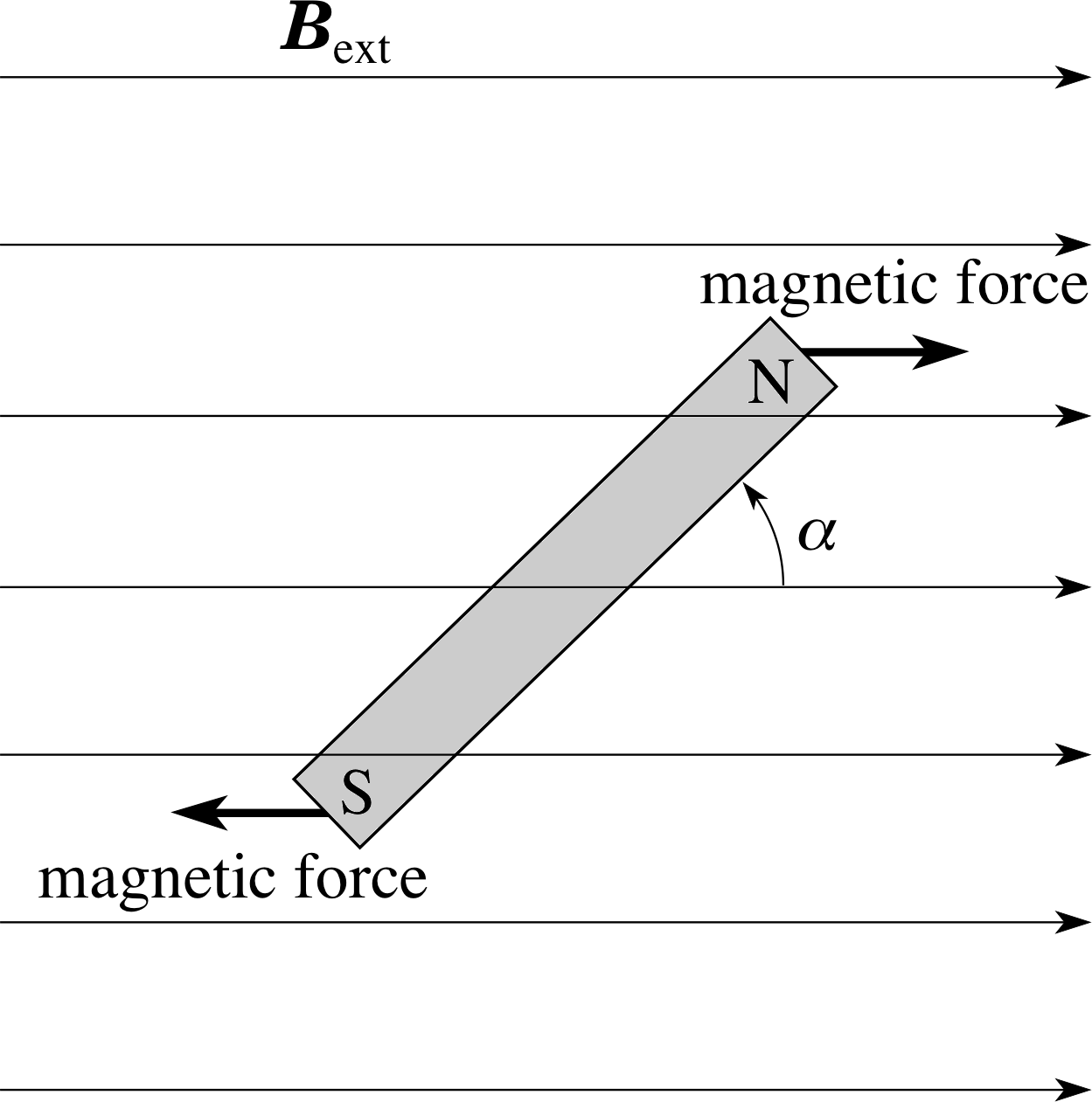
Figure 12 When a small bar magnet is in a uniform external magnetic field Bext, the magnet tends to align itself with the direction of the magnetic field. This is why compass needles align themselves to point in the direction of the Earth’s magnetic field.
As far as its magnetic effect is concerned we can represent an atomic electron by an equivalent tiny bar magnet that produces a magnetic field of the appropriate strength. We shall now discuss the effect of an externally applied magnetic field on this tiny bar magnet and this discussion will lead to an understanding of the magnetic quantum number.
A small bar magnet in an externally applied magnetic field Bext will tend to align itself with the direction of the external magnetic field, as shown in Figure 12. If the magnet is initially aligned with the external magnetic field then work must be done (i.e. energy transferred to the bar magnet) in order to change that alignment. So, if the magnet is pointing at an angle different from α = 0, it is a source of stored magnetic potential energy. This energy is greatest when α = 180°. Because of the analogy between the bar magnet and an atomic electron with orbital angular momentum L, we are not surprised to find that the electron also possesses a magnetic potential energy that depends on the orientation of L relative to the external magnetic field Bext.
Thus, the orientation of the orbital angular momentum vector will affect the energy of a quantum state when it is subject to an external magnetic field.
Now let us apply these ideas to the electrons in the p subshell of an atom. We know that a p subshell can accommodate up to six electrons, and that these electrons normally have identical energies (i.e. they all have the same threshold energy). But what happens to these electrons when a magnetic field is applied?
For example, consider an atom of magnesium, whose ground state configuration is 1s2 2s2 2p6 3s2. In the ground state the 3s subshell of this atom is full and the lowest unoccupied level is the 3p subshell. If magnesium atoms are heated sufficiently a significant number of them will be excited out of their ground state, and in many cases the excited atom will have an electron in the 3p subshell and a corresponding vacancy in the 3s subshell. Observations of the emission spectrum from hot magnesium vapour, in which many atoms have been excited in this way, reveal an intense spectral line of frequency 1.05 × 10¹⁵ Hz caused by atoms making the transition from the excited state with the partly occupied 3p subshell, back to the ground state, in which 3p is empty but 3s is full.
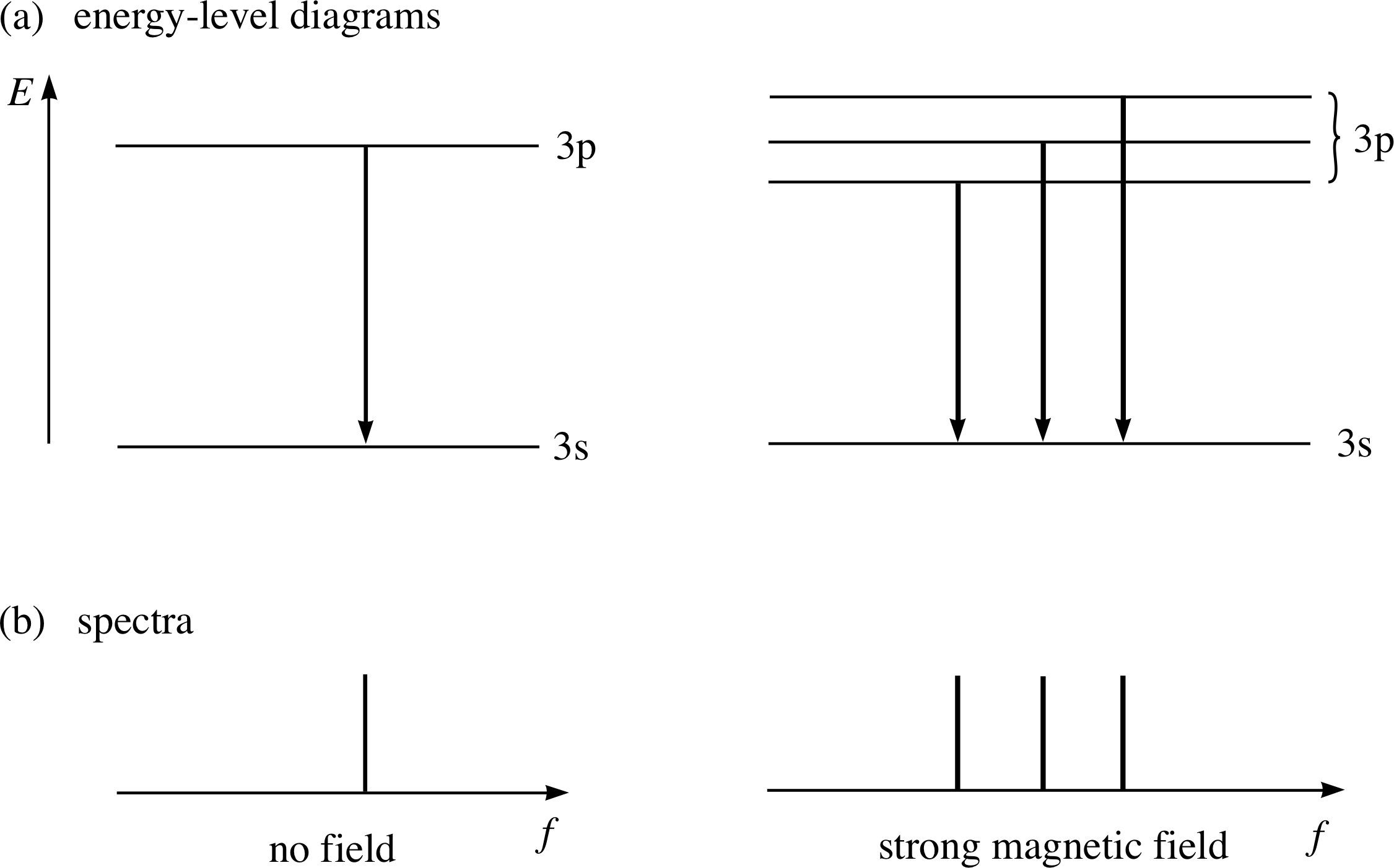
Figure 13 Splitting of the p to s transition for magnesium in a strong magnetic field. Note that in the right–hand diagrams the extent of the splitting is exaggerated for the sake of clarity.
This transition and the spectral line that corresponds to it in the absence of any external magnetic field, are shown on the left in Figures 13a and 13b.
In 1896 the Dutch physicist Pieter Zeeman (1865–1943) demonstrated that something remarkable happened to this sort of spectral line when the atoms were subjected to a magnetic field: the line splits into three closely spaced lines (shown on the right in Figure 13).
This phenomenon, known as the Zeeman effect, indicates that in the presence of a magnetic field either the 3s or 3p levels (or both) split into several levels with slightly different energies. As we will see later it is the 3p level here which splits into three levels, and the three spectral lines observed correspond to transitions from each of these to the single (unsplit) ground state. i The magnetic field is said to ‘split the 3p level’.
In view of our earlier discussion of bar magnets, current loops and stored magnetic energy it is pretty clear that we can interpret this three–fold splitting as an indication that the orbital angular momentum associated with a p subshell can be orientated in one of three ways relative to the direction of the external magnetic field.
In the absence of the magnetic field these orientations have no effect on the energy so they all correspond to a single energy level and are said to be degenerate. The application of an external magnetic field is said to ‘lift the degeneracy’. The different orientations then correspond to slightly different energies and deserve to be distinguished from one another as belonging to distinct quantum states.
Later experiments confirmed that all levels corresponding to non–zero angular momentum (p, d, f, etc.) are split by an applied magnetic field. The fact that energy levels corresponding to particular values of n and l may be split in this way clearly indicates the need for at least one more quantum number. The new number is called the orbital magnetic quantum number ml, an appropriate name because, within a given shell, energy levels corresponding to the same l but different ml are distinguished in the presence of a magnetic field.
As usual, quantum mechanics limits the possible values that ml may take. In a subshell with orbital angular momentum quantum number l, the only possible values of the orbital magnetic quantum number are the integers between +l and −l inclusive. Thus the three quantum states, that the Zeeman effect reveals within any p subshell (l = 1), correspond to the values ml = +1, ml = 0 and ml = −1 i
✦ What values of the orbital magnetic quantum number identify the following:
(a) the one quantum state in an s subshell;
(b) the five quantum states in a d subshell?
✧ (a) Because this subshell corresponds to l = 0, the subshell has only one associated value, ml = 0.
(b) The d subshell corresponds to l = 2 and therefore has five associated values of ml :
ml = +2, ml = +1, ml = 0, ml = −1 and ml = −2
(Remember, the ml values span all the integers between +l and −l inclusive.)
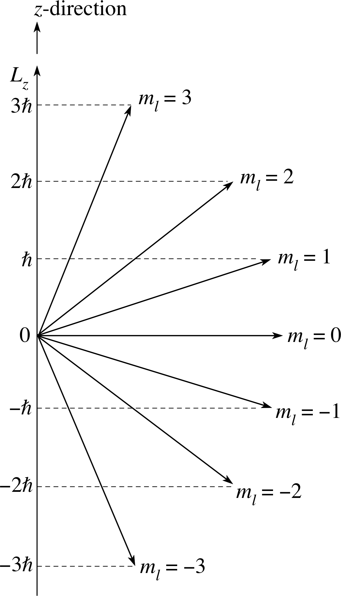
Figure 14 When the electron has the orbital angular momentum quantum number l = 3, its angular momentum vector L can be inclined at any one of seven possible angles to an arbitrarily defined z–axis. The z–component Lz can have the values $3\hbar$, $2\hbar$, $\hbar$, 0, $-\hbar$, $-2\hbar$, or $-3\hbar$.
We have already said that the different values of ml correspond to different orientations of the orbital angular momentum L, but it is possible to give it an even more precise meaning if we are willing to delve further into the complexities of quantum mechanics. According to quantum mechanics, if you arbitrarily choose a direction and call it the z–axis of a Cartesian coordinate system, and if you then measure the z–component Lz of the orbital angular momentum L of a bound electron, you will find that the result is quantized, just like the energy and the magnitude of the orbital angular momentum. In fact, in a subshell with orbital angular momentum quantum number l the only allowed values of the z–component of the orbital angular momentum are:
$L_z = m_l\hbar$ with ml = +l, l − 1, ... −(l − 1), −l(3)
The implications of this restriction for an f quantum state in which l = 3 are shown in Figure 14. The angular momentum vector, which must have magnitude $L = \sqrt{12\os}\hbar$ in this case, can only have one of seven values for Lz from $L_z = 3\hbar$ to $L_z = -3\hbar$ through all integer steps of $\hbar$. We can represent this diagramatically by putting the vector L at one of seven orientations with respect to the positive z–axis. Of course, so far as the atom is concerned, there is nothing special about this z–direction, which was chosen arbitrarily. This means that the z- component of the angular momentum of an atomic electron will be given by $m_l\hbar$, whatever direction is chosen to be the z-axis. This is a deeply counter–intuitive result that can only be fully understood in quantum mechanical terms, but it is experimentally verified.
✦ If the orbital angular momentum quantum number of an electron in a hydrogen atom is known to be l = 3, what are the possible results of an experiment to measure the z–component of the orbital angular momentum L of this electron?
✧ A measurement of the z–component of the electron’s angular momentum vector will give one of the results:
$-3\hbar$, $-2\hbar$, $-\hbar$, 0, $+\hbar$, $+2\hbar$, or $+3\hbar$, corresponding to one of the allowed values of ml.
(Remember the values of ml span the integers between +l and −l inclusive.)
The magnitude L of the orbital angular momentum of a bound electron is quantized, as is the z–component of the angular momentum vector L. The allowed values of L are determined by the orbital angular momentum quantum number l, and are given by
$L^2 = l(l + 1)\hbar^2$ with l = 0, 1, 2, ... n − 1(Eqn 2)
The allowed values of Lz are determined by the orbital magnetic quantum number ml
$L_z = m_l\hbar$ with ml = +l, l − 1, ... −(l − 1), −l(Eqn 3)
Before we leave this strange quantum mechanical result we must point out another non–intuitive feature which emerges from the quantum model. i We have seen that the angular momentum can be defined in terms of its magnitude L and its z–component Lz. You might also have expected that we could say something about the other two components of angular momentum, Lx and Ly, especially as we have been speaking of the orientation of the vector L.
The truth is that we can say nothing about Lx and Ly according to quantum mechanics! Once we have defined L by L and Lz, that is all we can know. Lz It is rather misleading then to say that we know the orientation of L where this term would imply that we also knew Lx and Ly. All we know is the projection of L along a chosen axis, not its orientation. We can use Figure 14 to visualize this if, for each ml case, we think of the angular momentum vector as lying anywhere on the surface of a cone obtained by rotating the diagram around the z–axis. In this three–dimensional representation Lx and Ly can have any values, but Lz stays fixed. (Of course Lx and Ly are restricted in that L2 = Lx2 + Ly2 + Lz2 and so we know that (Lx2 + Ly2) = L2 – Lz2, but we do not know Lx or Ly separately.)
4.3 The Stern–Gerlach experiment and electron spin
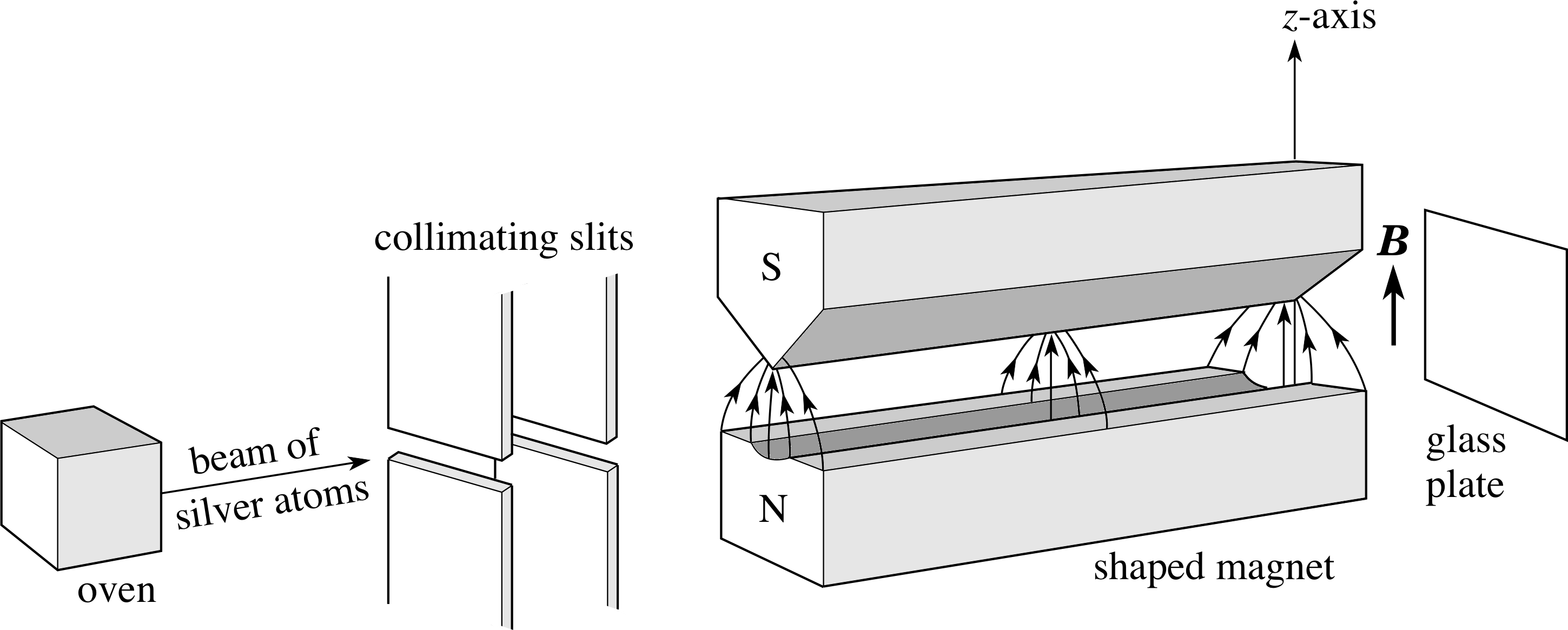
Figure 15 Schematic diagram of the Stern–Gerlach apparatus.
In 1921 the German physicist Otto Stern (1888–1969) and his colleague Walter Gerlach (1889–1979) carried out one of the most famous experiments in atomic physics. This became known as the Stern–Gerlach experiment. Their apparatus (Figure 15) enabled a carefully collimated i beam of silver atoms to pass through a non–uniform magnetic field that was everywhere perpendicular to the direction of the beam. Stern and Gerlach determined the distribution of the silver atoms after they had passed through this field by collecting the atoms on a glass plate at the far end of the apparatus.
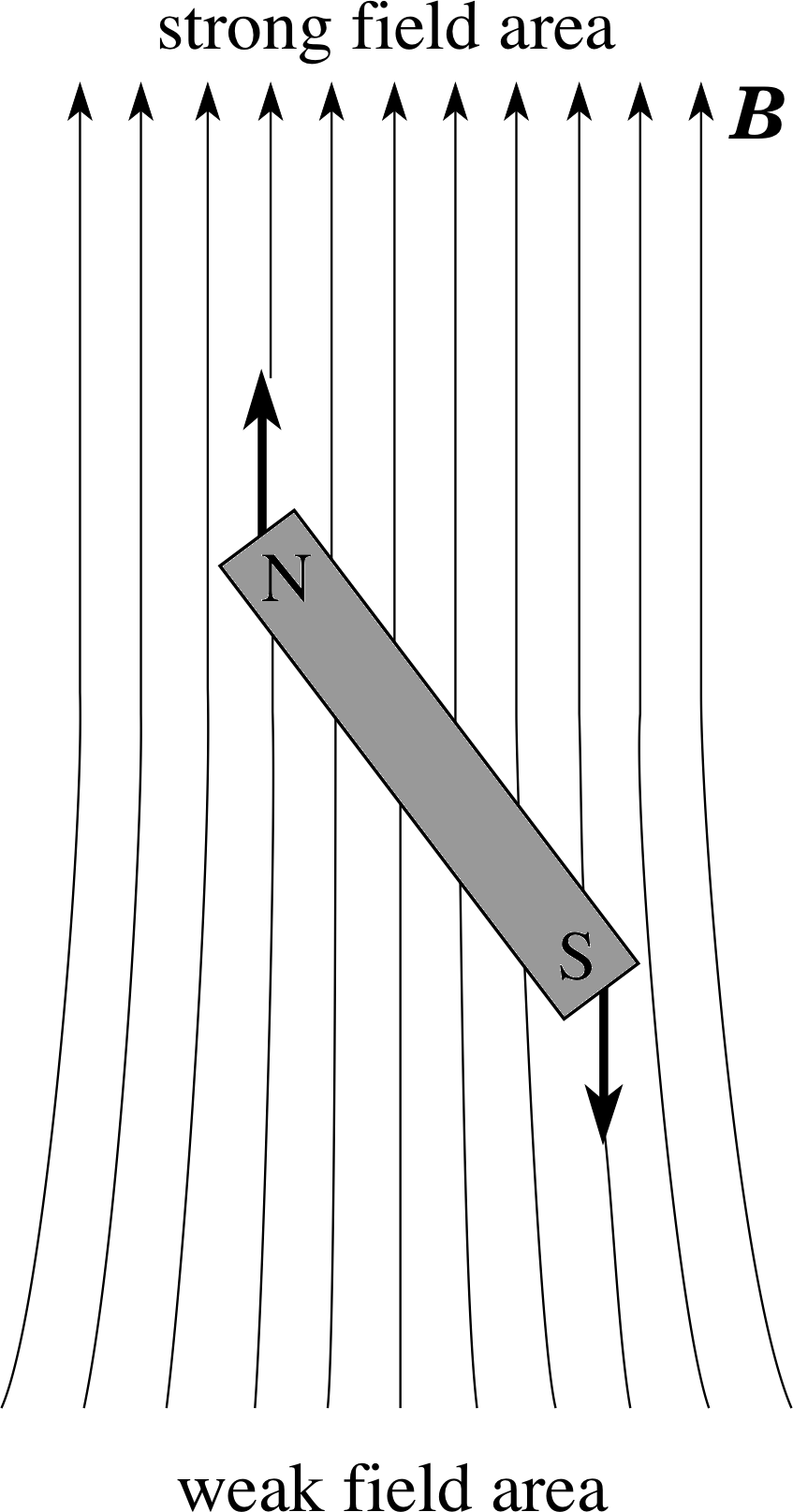
Figure 16 The effect of a non–uniform magnetic field on a bar magnet. The force acting on the north pole of this magnet is stronger than the force acting on its south pole, because the north pole is in a stronger field than the south pole. So there is a net force on the magnet (which also turns in the field). In the case shown here, the net force tends to move the magnet upwards, towards the top of the page.
In order to understand the significance of the Stern–Gerlach experiment it is helpful to think of each silver atom in the beam as a tiny bar magnet, just as we did in the last subsection. A bar magnet generally experiences a net force when it is moving through a non–uniform field (Figure 16), which tends to deflect it from its original direction of motion. This deflecting force will have a magnitude that depends on the magnetic field and the strength of the atomic magnet. The direction of the force is determined by the direction of the external field gradient and the orientation of the atomic magnet. For the magnet oriented as in Figure 16, the direction of the net force on the magnet is towards the increasing field direction, i.e. along the direction of the field gradient.
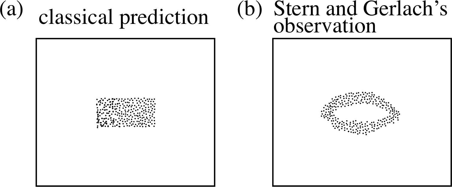
Figure 17 The outcome of the Stern–Gerlach experiment: (a) as predicted by classical physics, (b) as observed by Stern and Gerlach.
If you didn’t know much about atoms, and you were totally unaware of quantum mechanics, you might expect that the atoms really would behave just like tiny, randomly orientated bar magnets and that they would produce some sort of vertical smear on the glass plate (Figure 17a) as all orientations of the atomic magnets are possible. Of course, you already know something about quantum mechanics so you might suspect that the orbital angular momentum of the ground state configuration would determine the magnetic properties of the atom. Silver is an interesting choice of beam substance, because its ground state configuration is:
Ag 1s2 2s2 2p6 3s2 3p6 3d10 4s2 4p6 4d10 5s
A filled shell produces no net magnetic property since all ml values are present, and these are symmetric about ml = 0. We might then expect the magnetic property of silver atoms to be determined by the single electron in the n = 5 shell. Since this has l = 0 and ml = 0 (5s electron) we expect no magnetic property and so predict that the beam does not split. This is also wrong. What was actually seen is indicated in Figure 17b. As Stern and Gerlach found, the beam of silver atoms was split into two components.
Although the beam was not split in the absence of the inhomogeneous magnetic field, there was a clear splitting when that field was applied. The implication is that the silver atom does behave like a tiny magnet, but the associated angular momentum vector of the atomic magnet only has two possible orientations relative to the direction of the external magnetic field.
✦ Is there any value of the orbital angular momentum quantum number l that would correspond to just two allowed orientations of the angular momentum vector L?
✧ No. For any given value of l there are always 2l + 1 possible values of ml (from +l to −l in integer steps) and hence 2l + 1 possible orientations. This must be an odd number for any integer value of l.
A satisfactory explanation for the Stern–Gerlach results came in 1925 from the work of two young graduate students working in Leiden, Samuel Goudsmit (1902–1978) and George Uhlenbeck (1900–1988). They suggested that the electron itself has an intrinsic angular momentum, as well as the more familiar properties of mass and charge. This intrinsic angular momentum of the electron, or spin_angular_momentumspin as it is called, is quite independent of any orbital angular momentum that the electron might have due to its motion about the nucleus. Moreover, their arguments required that the spin angular momentum vector should have only two possible orientations in an external magnetic field. i
Using the idea of spin, the results of the Stern–Gerlach experiment can be explained as follows. Each silver atom contains 47 electrons, and it turns out that the vector sum of the orbital and spin angular momenta for 46 of these electrons is zero. Moreover, the remaining electron has zero orbital angular momentum since it is an s quantum state. Hence, the net angular momentum for a whole silver atom can be attributed solely to the spin angular momentum of a single electron.
In the Stern–Gerlach experiment, the beam splits up into two components simply because the electron’s spin angular momentum can have only two possible orientations in an external magnetic field.
4.4 The spin and spin magnetic quantum numbers
Experiments have shown that the electron is not alone among subatomic particles in having spin. Neutrons and protons also have two spin states in an external magnetic field.
The quantum number that determines the magnitude of the spin angular momentum of any subatomic particle is denoted by s and is called its spin angular momentum quantum number. Quantum mechanics tells us that the magnitude S of the spin angular momentum vector S of the particle is related to its spin angular momentum quantum number s by the equation
$S^2 = s(s+1)\hbar^2$(4)
Each particle has a particular value of s, which specifies an intrinsic property of the particle, analogous to its charge and mass. For any electron, whether or not it is part of an atom, s = 1/2.
✦ What, then, is the magnitude of the spin angular momentum of the electron?
✧ Using the above equation,
$S = \sqrt{(1/2)[(1/2)+1]\os}\hbar = \sqrt{3\os}\hbar/2$
The spin angular momentum vector S of an electron can have two possible orientations with respect to an arbitrary z–axis. These orientations are specified by the electron’s spin magnetic quantum number ms, which can have only two values +1/2 and −1/2. Hence:
$S_z = m_s\hbar$ with ms = +1/2, −1/2(5)
In other words, the z–component of the spin angular momentum vector of an electron – any electron, not only those in atoms – can have one of two values, $+\hbar/2\text{ or }-\hbar/2$.
✦ If the Stern–Gerlach experiment is repeated with helium atoms, it is found that they are not deflected by the non–uniform field. Given that the helium atoms each contain two electrons in the 1s level, how can this phenomenon be explained?
✧ The behaviour demonstrates that helium atoms are not magnetic. This absence of magnetism can be explained only by assuming that the two electron ‘magnets’ have opposite polarity, so that they cancel each other out. In other words, the two electrons in the n = 1 shell must have opposed spin orientations, one corresponding to ms = 1/2, the other to ms = −1/2. We say that the spins are paired.
The existence of paired electrons of this sort is an important phenomenon. In general it turns out that atoms containing only full shells (or subshells) of electrons have no magnetic properties due to orbital or spin angular momentum. This means that all electron spins must be paired when a shell (or a subshell) is full.
In presenting evidence about the interaction of electrons with externally applied magnetic fields, we have been careful to choose the simplest cases. For example, we were careful to avoid discussion of the effect of a magnetic field on the p to s transition in an atom like sodium (ground state configuration 1s2 2s2 2p6 3s), where the atom has a magnetic effect due to the spin of the unpaired electron. It was partly in this sense that we ‘simplified’ our earlier discussion of the Zeeman effect.
Magnetic effects associated with spin angular momentum can combine with those due to orbital angular momentum to produce highly complex splitting patterns for spectral lines from most atoms in a magnetic field. In the examples we have chosen, magnetic effects are due either to spin (Stern–Gerlach) or to orbital motion (Zeeman effect) but not a combination of both.
4.5 The four quantum numbers and the Pauli exclusion principle
We can now describe each electron in an atom completely by means of four quantum numbers. The names and allowed values of these quantum numbers are shown in the box below.
The principal quantum number, nn = 1, 2, 3...
The orbital angular momentum quantum number, ll = 0, 1, 2... (n − 1)
The orbital magnetic quantum number, mlml = −l... 0... +l
The spin magnetic quantum number, msms = ± 1/2 i
Each atomic electron has its own set of these four quantum numbers, which specify the electron’s quantum state. A question that naturally arises is ‘How many electrons can occupy a given quantum state?’ or, in other words, ‘How many electrons can share the same set of values for all four quantum numbers?’ This question was answered in 1924 by the Austrian physicist Wolfgang Pauli (1900–1958) using a simple but extremely powerful principle that is one of the cornerstones of atomic physics and is called the Pauli exclusion principle:
The Pauli exclusion principle:
No two electrons in an atom can simultaneously occupy the same quantum state, so the quantum state for an atom must have separate distinct quantum states for each of its electrons.
It follows from this that no two electrons in an atom can possibly have the same values for all four quantum numbers. For example, if it is known that two atomic electrons occupy 1s states in an atom and therefore are characterized by the quantum numbers n = 1, l = 0, ml = 0, then the Pauli exclusion principle tells us that they must have different spin orientations (ms = +1/2 and ms = −1/2) in order that their complete sets of four quantum numbers are not the same.
We saw in Subsection 3.1 that a subshell characterized by orbital angular momentum quantum number l can contain up to 2(2l + 1) electrons. Our statements about the allowed values of the various quantum numbers, together with the Pauli exclusion principle, explain the origin of this limitation, as the next question will enable you to show.
Question T8
Using the appropriate quantum numbers, list all the quantum states that could comprise the l = 3 subshell of the n = 4 shell of an atom. Confirm that there are 2(2l + 1) of these states.
Answer T8
For each of these quantum states n = 4 and l = 3, the allowed values of ml and ms are then (3, 1/2), (3, −1/2), (2, 1/2), (2, −1/2), (1, 1/2), (1, −1/2), (0, 1/2), (0, −1/2), (−1, 1/2), (−1, −1/2), (−2, 1/2), (−2, −1/2), (−3, 1/2), (−3, −1/2).
There are 14 quantum states in all, in agreement with the rule that there should be 2(2l + 1).
Each of the quantum states in an atom corresponds to a unique wavefunction and each has a definite energy. The fact that different quantum states may be associated with the same energy offers deeper insight into the nature of degeneracy.
4.6 Explaining ground state electronic configurations
We are now in a position to draw together the ideas that we have developed about atomic energy levels and quantum numbers in order to establish the electronic configurations of the elements.
At this stage you should be able to write the ground state electronic configuration of the atom of any element up to atomic number 18, argon, using the appropriate sequence of electron subshells (1s, 2s, 2p, 3s, 3p) and remembering the degeneracy of the levels.
To do this you follow the guidelines 1 to 6 set out in the box below.
- 1
-
In the ground state the electrons fill the lowest energy states first.
- 2
-
The electron shells are labelled in sequence by the principal quantum number 1n, which can have values 1, 2, 3, etc.
- 3
-
The electron shells designated by the principal quantum number are divided 0into subshells, designated by the orbital angular momentum quantum number, l.
- 4
-
The number of subshells in a shell is equal to the value of the principal quantum number (because l has values 0, 1, 2, ... n − 1).
- 5
-
Within an electron shell, the energies of the subshells increase with the value of the orbital angular momentum quantum number l.
- 6
-
There is a maximum number of electrons that any subshell can hold:
- l = 0, s quantum state: two electrons
- l = 1, p quantum state: six electrons
- l = 2, d quantum state: ten electrons
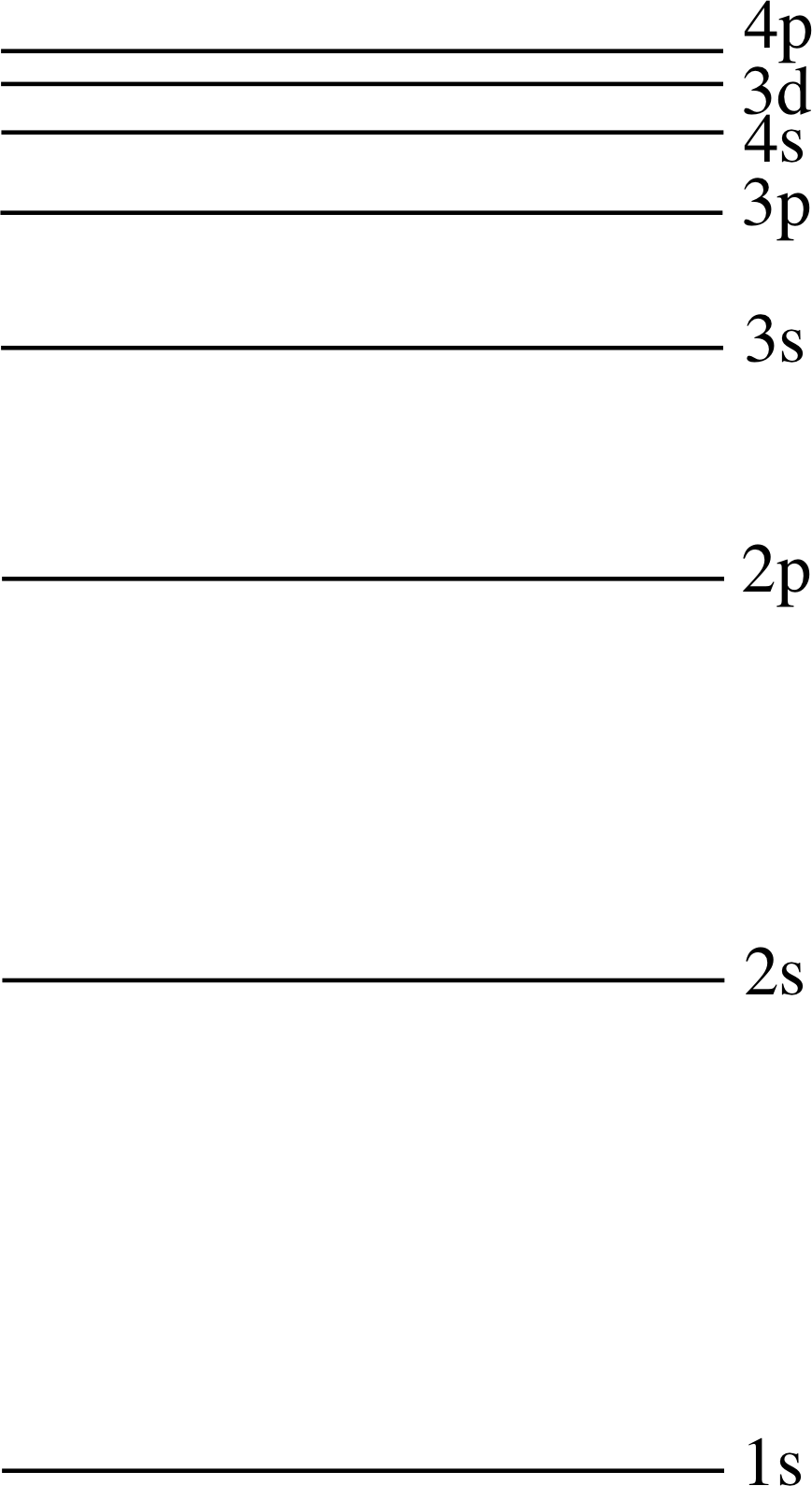
Figure 18 The electron energy level diagram up to the 4p subshell.
So much for the first 18 elements, but what about the rest? You will recall from Subsection 3.3 that in the case of potassium (Z = 19) the 4s subshell starts to fill before the 3d. Manganese (Z = 25) shows similar behaviour with a full 4s subshell even though there are only five electrons in the 3d subshell. It is usual to represent this state of affairs by writing the ground state electronic configuration as follows:
Mn 1s2 2s2 2p6 3s2 3p6 4s2 3d5
As we explained earlier this indicates that the energy associated with the two 4s states is less than that associated with the five 3d states, as can be clearly seen from a typical energy level diagram shown in Figure 18. The reason for this behaviour (as discussed earlier) is that the energy of the 3d subshell relative to the 4s subshell depends on interactions between the electrons in the atom. These can be very difficult to work out and generally depend on the total number and distribution of the electrons that are present.
In representing the electronic configuration of an element in the way shown above for manganese, you indicate how the electrons occupy the energy levels and also what is the outer shell structure of the atom. It is this outer shell structure which determines most of the atom’s physical and chemical properties, as is discussed elsewhere in FLAP under the description of the periodic table. This notation does not provide any information about the magnetic quantum numbers which can be important in determining the order in which states are occupied. This information can be provided by representing the quantum state of the atom as a series of boxes, and by representing the electrons as arrows pointing up or down to indicate the spin orientations.
To take one of the simplest cases, helium, the 1s subshell is represented by a single box, and two half–headed arrows represent the electrons: i
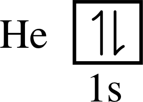
Notice that this notation vividly shows the pairing of the electrons in the 1s subshell of helium. Another example of this box notation of electronic configuration refers to the magnesium atom, which has the electronic structure 1s2 2s2 2p6 3s2, and is represented by:
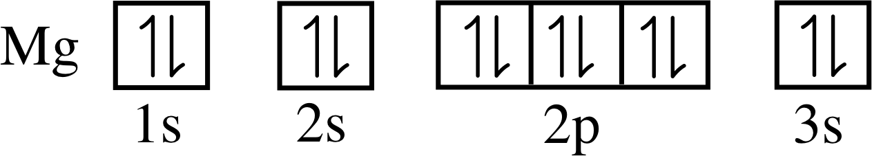
Notice that the electron spins are paired within each full box. Also, note that there are single boxes for 1s and 2s, because they each contain only one pair of electrons, and there is a triple box for 2p because this subshell is triply degenerate in ml.
✦ Use this notation to write down the electronic structure of argon (Z = 18).
✧ The electronic structure of argon is 1s2 2s2 2p6 3s2 3p6:
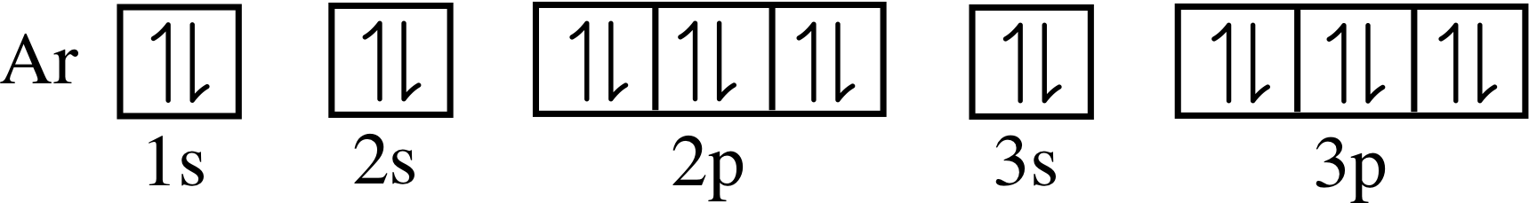
✦ Now use the box notation to try to write out the electronic configuration of sulphur, which has atomic number 16. The order of filling the subshells is 1s, 2s, 2p, 3s, 3p, and the electronic structure is 1s2 2s2 2p6 3s2 3p4.
Here are the boxes labelled up to 3p:
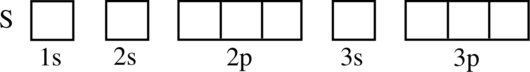
✧ You should have been faced with a dilemma when you attempted to put the arrows in your 3p boxes. Is there any way of deciding whether to write
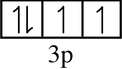 or
or 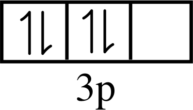 ?
?
That is, should the electrons be paired, as on the right, or be left unpaired if possible, as on the left?
Figure 19 The order in which the subshells are filled for atoms in their ground states.
The results of experimental determinations of electronic configurations by spectroscopy show that this question can be answered by an empirical rule known as Hund’s rule:
Within any subshell, there will be the maximum number of unpaired electrons in an atom in its ground state. i
Therefore the left–hand version is correct in this case,
or ?
because it shows two unpaired electrons whereas there are none in the right–hand version.
Now, with this rule, you should be able to write the ground state electronic structure of the atoms of any element, given the correct sequence of subshells. Figure 19 conveniently shows the order in which the subshells are filled: you simply follow the snake.
Question T9
Find the electronic configurations of ground state atoms of phosphorus (15), zinc (30) and cobalt (27), using both the s-p-d-f notation and the box notation (atomic numbers are shown in brackets). Use the sequence of subshells in Figure 19 and remember to fill the subshells of lowest energy first.
Answer T9
The configurations and box structures are:
P 1s2 2s2 2p6 3s2 3p3
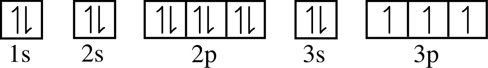
Zn 1s2 2s2 2p6 3s2 3p6 4s2 3d10
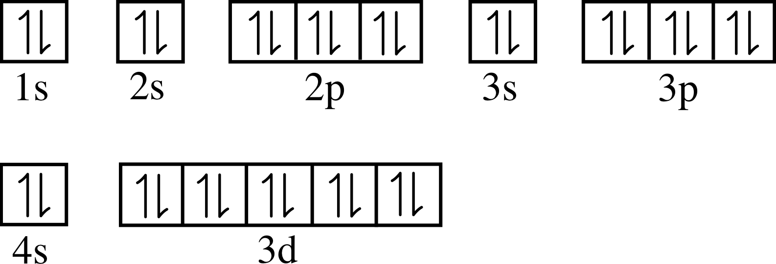
Co 1s2 2s2 2p6 3s2 3p6 4s2 3d10
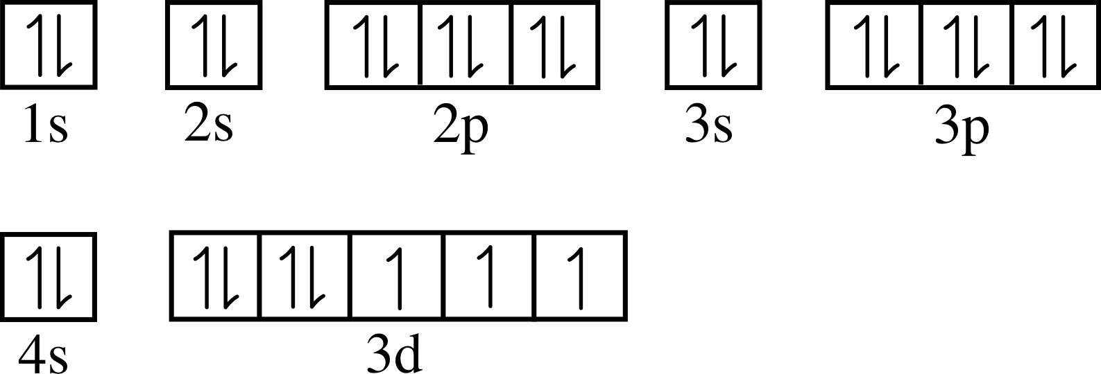
✦ Now write down the structure of chromium, which has atomic number 24.
✧ If you have correctly interpreted the guidelines, you will have predicted the configuration:
1s2 2s2 2p6 3s2 3p6 4s2 3d4
As we shall soon see this is not the right answer.
It turns out that a few elements do not obey the guidelines precisely. i In atoms with many electrons, the energies of the outer subshells are sometimes very close together indeed, as you can see from Figure 18, and occasionally the presence of electrons in say, the 3d subshell changes the relative energy of the 4s subshell, so that sometimes it contains two electrons and sometimes only one. This sort of information is obtained from a detailed examination of the atomic spectra of elements, which shows the electronic configuration of chromium to be:
Cr 1s2 2s2 2p6 3s2 3p6 4s1 3d5
Clearly, from the unexpected electronic configuration of chromium, the energies of the configurations must be very similar. Knowing the answer, one can look for sensible reasons for it. To predict it would have been much more difficult, but it is possible using advanced techniques in quantum mechanics.
5 X–ray spectra
5.1 The two components of X–ray spectra
On Friday 8 November 1895, a discovery was made that was to puzzle physicists and to defy complete explanation for almost twenty years. The physicist, Wilhelm Röntgen (1845–1923), was experimenting in his laboratory with an evacuated tube in which charged particles (later identified as electrons) were accelerated from one electrically charged plate to another. He found to his amazement that when these particles impinged on the wall of the tube, rays were emitted that caused some nearby crystals to glow (this is an example of fluorescence).
Röntgen made a thorough investigation of the new rays, which he called X–rays, and nearly two months elapsed before he submitted his results for publication. During that time, he took the first X–ray photographs, one of which showed the bones in one of his wife’s hands.
X–rays are a form of electromagnetic radiation. They have very short wavelengths (roughly between 0.003 nm and 30 nm), and, in common with all forms of electromagnetic radiation, their energy is emitted and absorbed as photons.
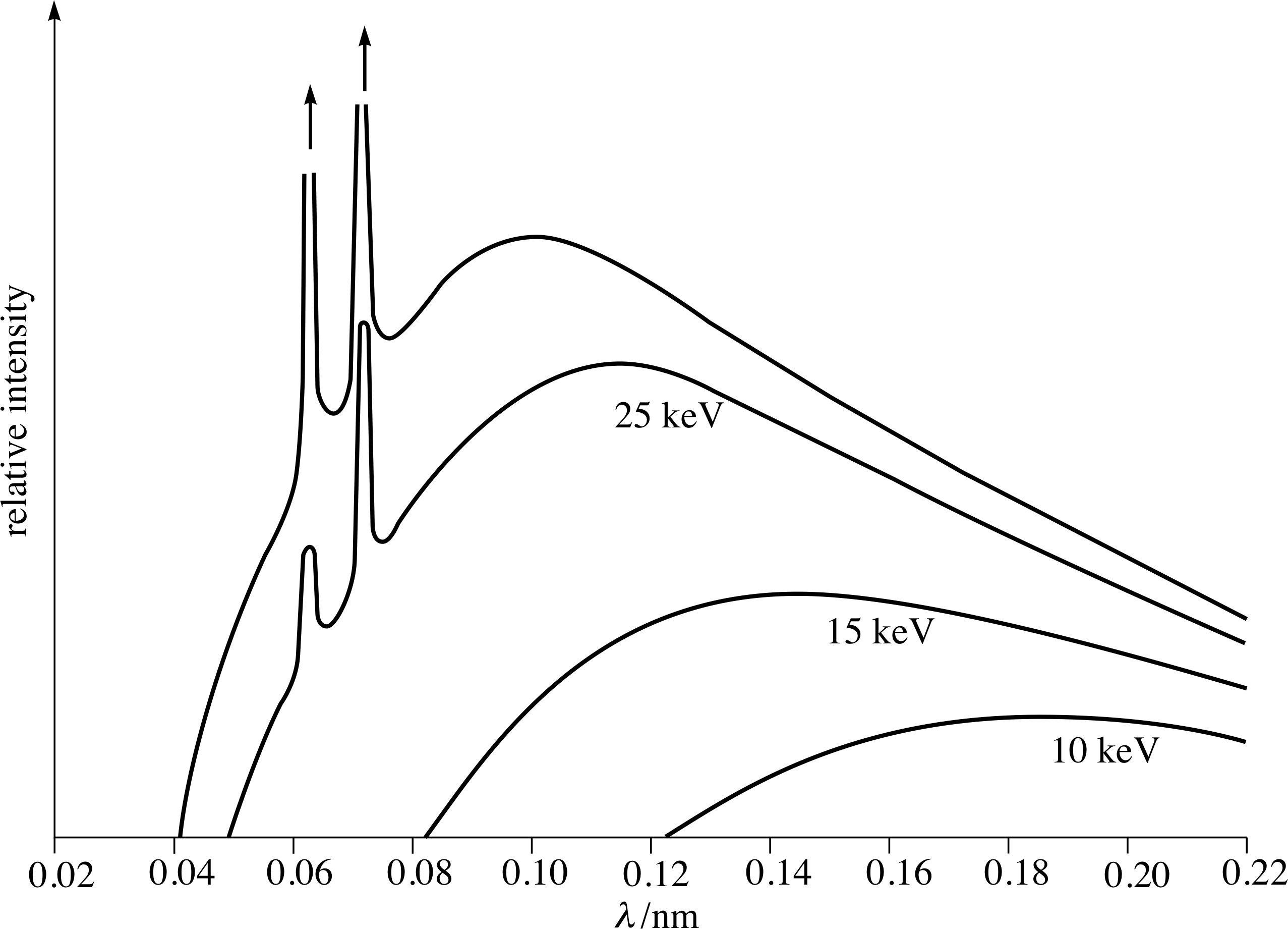
Figure 20 The X–ray spectrum of molybdenum between λ = 0.02 nm and 0.22 nm shown for different acceleration voltages.
Figure 20 shows the X–ray spectra of the element molybdenum; the X–rays are emitted when a molybdenum target is bombarded by electrons that have been accelerated through a potential difference of several thousand volts. From Figure 20 you can see that at low accelerating voltages the X–ray spectrum is continuous_x_ray_spectrumcontinuous, whereas at high voltages we see some spikes in the intensity, which is evidence of the emission of characteristic_x_ray_spectrumcharacteristic X–rays by the bombarded target.
Consider first the continuous X–ray spectrum. If the incident electrons have been accelerated through a potential difference V, their kinetic energy as they strike the target will be eV, where e is the magnitude of the charge of the electron. As they are being brought to rest within the target, we would expect that the electrons will have a range of kinetic energies from zero to eV. Electrons that pass close to the nucleus of one of the molybdenum atoms will be deflected and lose some kinetic energy, which will appear as the energy of an X–ray photon. Radiation produced in this way is called bremsstrahlung – ‘braking radiation’ in German. All electrons (whose kinetic energies lie in the range from 0 to eV) can produce bremsstrahlung, and in this way contribute to the continuous X–ray spectrum.
A prominent feature of the continuous spectrum is the sharply defined cut–off wavelength λmin, below which there is no continuous spectrum. This minimum wavelength corresponds to an encounter in which one of the incident electrons loses all of its initial kinetic energy eV in one go, radiating it away as a single X–ray photon. The wavelength associated with this photon, the minimum possible X–ray wavelength, is found from
eV = hf = hc/λmin
and hence λmin = hc/eV
This cut–off wavelength depends on the applied voltage but is independent of the target material. If you were to switch from a molybdenum to a copper target, all features of Figure 20 would change except the cut–off wavelength.
In contrast, the wavelength of the characteristic_x_ray_spectrumcharacteristic X–rays, represented by the sharp intensity peaks, certainly does depend on the target material. The emission of characteristic X–rays is analogous to the emission of visible spectral lines; both kinds of emission are due to transitions between the energy levels of electrons in atoms. However, there are important differences between the two phenomena.
X–rays have a much shorter wavelength than visible light. Characteristic X–rays are emitted from a heavy atom when an ejected inner–shell (low energy) electron is replaced by an outer–shell (high energy) electron. In this case the spacing between the two energy levels is thousands of electronvolts. This is in contrast to the typical energy differences of ≈ 2 eV, which give rise to visible light emission (λ = 400–750 nm).
5.2 X–rays and atomic numbers
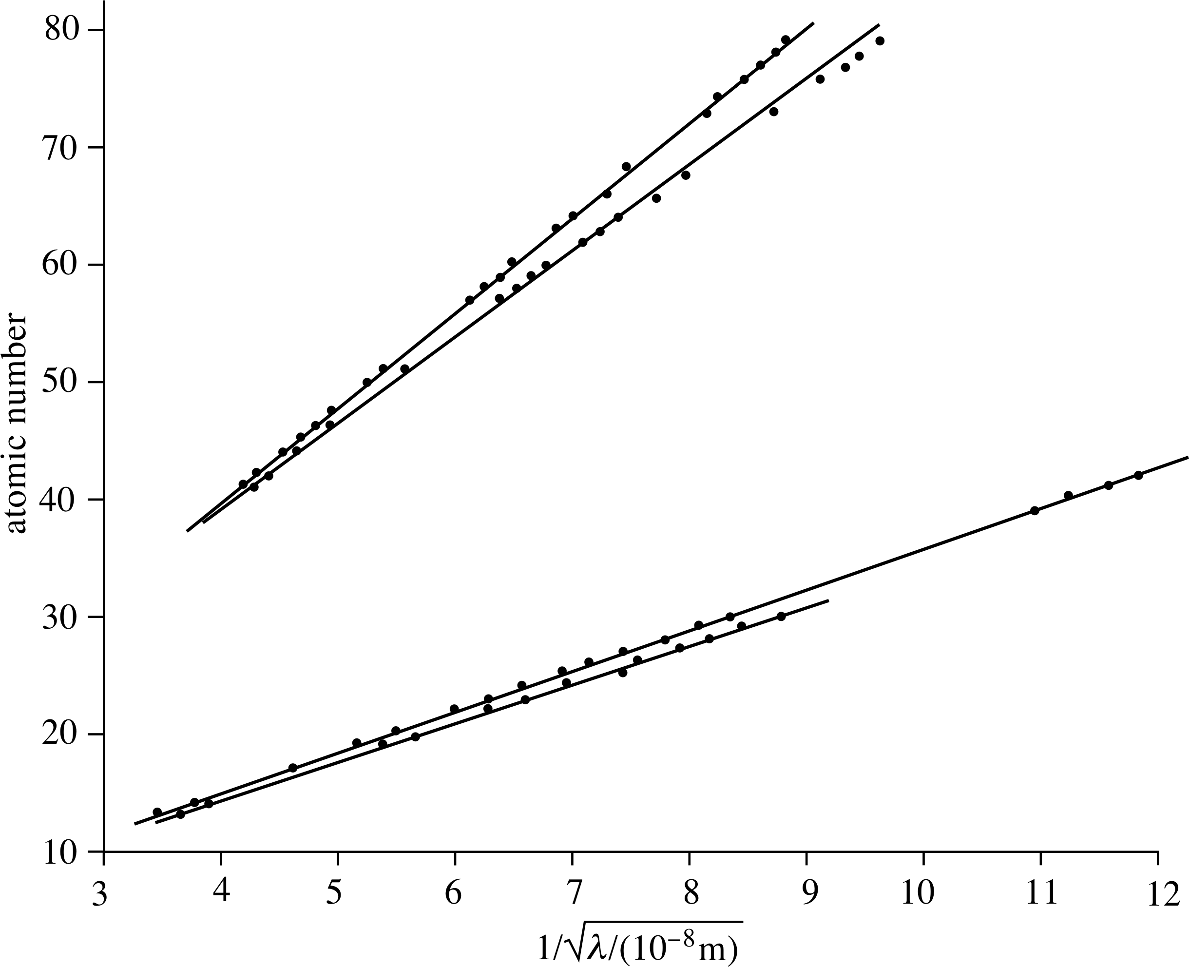
Figure 21 Moseley found that there was a linear relationship between the atomic numbers of heavy elements and the reciprocal of the square roots of the wavelengths of their most intense characteristic X–ray lines (Z ∝ λ−1/2). Four series of lines are shown in this figure.
An important contribution to the study of X–rays was made by Henry Moseley (1887–1915).
Moseley’s work was carried out before the concept of atomic number had been developed, at a time when chemists and physicists listed elements in order of their atomic weight (which we would now call their relative atomic mass). He investigated the relationship between the frequencies of the most intense characteristic X–rays emitted by heavy elements and their atomic weights. Moseley found that for the heavy elements the reciprocal of the square root of the wavelength of the most intense characteristic X–ray line was linearly related to a quantity which increased with atomic weight, but was not actually proportional to it (Figure 21).
He took this new quantity to represent the increasing number of electrons in the atom, which he correctly identified with the increasing positive charge of the nucleus. This new quantity subsequently came to be known as the atomic number Z. Thanks to this work it became clear that there were still a number of undiscovered elements, all of which have since been found, and also a few cases where elements were out of sequence in the periodic table, due to their unusual isotopic abundances modifying the atomic weights.
It is possible to understand Moseley’s conclusion qualitatively. If an electron in a heavy element falls down into a vacancy created in the innermost shell (n = 1) the energy change of the transition is dominated by the very large negative energy of the deep innermost shell. In many ways the transition is largely independent of all the other electrons and is very much like a transition of a single electron from an excited state of hydrogen down to the n = 1 shell, except for one very large difference. Since the nucleus of the heavy atom contains many more protons than that of hydrogen, this n = 1 shell is much closer to the nucleus than in hydrogen and so the energy change is much greater. In fact one can model this quite successfully by treating the heavy atom as a hydrogen atom but having a nucleus of charge (Z – 1)e, where Z is the atomic number. i
If the Bohr model for hydrogen is then used, but with a nuclear charge (Z – 1)e rather than e, then Moseley’s law emerges after some algebraic manipulation.
Figure 20 The X–ray spectrum of molybdenum between λ = 0.02 nm and 0.22 nm shown for different acceleration voltages.
Question T10
(a) Why is a continuous range of X–ray wavelengths emitted by a molybdenum target when it is struck by high energy electrons?
(b) Refer to Figure 20, and in particular to the X–ray spectrum that has the lowest cut–off wavelength. Calculate the accelerating voltage of the electrons bombarding the molybdenum target in this case.
Answer T10
(a) When the electrons strike the target, they slow down and emit electromagnetic radiation (bremsstrahlung): the kinetic energy of the electrons is converted into the energy of the radiation. Since the electrons lose different amounts of kinetic energy, the radiation emitted from the target has many different wavelengths. In other words, a continuous X–ray spectrum is emitted.
(b) The radiation with the shortest possible wavelength is λ′ emitted by electrons that are brought to rest in one collision with the target. In this case, the energy of the electron due to its acceleration through a potential difference of V volts is equal to the energy of the emitted photon
eV = hc/λ′ hence V = hc/eλ′
Since the cut–off wavelength λ′ is 0.041 nm:
$V = \rm \dfrac{(6.6\times10^{-34}J\,s)\times(3\times10^8\,m\,s^{-1})}{(1.6\times10^{-19}\,C)\times(4.1\times10^{-11}\,m)}$
Hence, the accelerating voltage V = 30 kV.
6 Closing items
6.1 Module summary
- 1
-
Studies of the Subsection 2.1successive ionization energies of atoms and Subsection 2.2photoelectron spectroscopy show that the energy levels of a multi–electron atom can generally be grouped into a number of shells which may be divided into subshells.
- 2
-
The electron shells are numbered 1, 2, 3, ... etc. This number is called the principal quantum number n. The shell with n = 1 is the most tightly bound.
- 3
-
The number of subshells in any given shell is equal to the principal quantum number of that shell. These subshells are labelled by the Subsection 4.1orbital angular momentum quantum number l, which may take integer values from 0 to n − 1.
- 4
-
The maximum number of electrons that can occupy a subshell with orbital angular momentum quantum number l is 2(2l + 1). The maximum number of electrons that can occupy a shell with principal quantum number n is 2n2.
- 5
-
Subshells with values of l equal to 0, 1, 2 and 3 are denoted by the letters s, p, d and f, respectively. These letters, in conjunction with the value of n, can be used as a shorthand way of labelling electron energy levels.
- 6
-
The magnitude L of the orbital angular momentum of a bound electron is quantized, as is its component in any specified direction, Lz.
- 7
-
The allowed values of L are determined by the Subsection 4.1orbital angular momentum quantum number l, and are given by
$L^2 = l(l + 1)\hbar^2$ with l = 0, 1, 2, ... n − 1(Eqn 2)
- 8
-
The allowed values of Lz are determined by the Subsection 4.2orbital magnetic quantum number ml, which thereby determines the orientational quantization
$L_z = m_l\hbar$ with ml = +l, l − 1, ... −(l − 1), −l(Eqn 3)
- 9
-
The electron itself has spin angular momentum, which can be oriented in one of two directions that are specified by the electron’s spin magnetic quantum number ms (ms = +1/2 or −1/2).
- 10
-
The Pauli exclusion principle states that no two electrons in an atom can occupy the same quantum state. Hence, no two electrons in the same atom can have the same set of four quantum numbers n, l, ml and ms.
- 11
-
It is quite possible for electrons in different quantum states to have the same characteristic energy. This is the phenomenon of degeneracy. In the presence of a magnetic field this degeneracy may be lifted, resulting in a splitting of the observed spectral lines. This is a manifestation of the Zeeman effect.
- 12
-
Using the four quantum numbers n, l, ml and ms and the Pauli exclusion principle, it is possible to write down the complete electronic configuration of an atom of an element in its ground state.
- 13
-
Hund’s rule states that in an atomic ground state, within each subshell, there will be the maximum number of unpaired electrons, consistent with the Pauli exclusion principle.
- 14
-
When a target is bombarded with electrons that have been accelerated through a potential difference of several thousand volts, X–rays are produced. The spectrum consists of two components: a continuous spectrum and characteristic spectrum. The characteristic spectrum is due to the replacement of ejected inner–shell electrons by outer–shell electrons, and the continuous spectrum is due to deceleration of the electrons.
- 15
-
There is a linear relationship between the heavy elements’ atomic numbers and the reciprocal of the square roots of the wavelengths of their most intense characteristic X–ray lines.
6.2 Achievements
Having completed this module, you should be able to:
- A1
-
Define the terms that are emboldened and flagged in the margins of the module.
- A2
-
Explain how the technique of photoelectron spectroscopy can be used to obtain information about the electronic structure of atoms.
- A3
-
Explain how the quantum state of each electron in an atom can be characterized by four quantum numbers.
- A4
-
Explain how empirical relationships between these quantum numbers can be used to determine the capacities of the electron shells and subshells.
- A5
-
Use these empirical rules, together with the s-p-d-f notation and Hund’s rule to write down the electronic structure of atoms in their ground states.
- A6
-
Outline the physical meaning of the four quantum numbers, n, l, ml, ms.
- A7
-
Explain the significance of the experiments of Zeeman and of Stern and Gerlach.
- A8
-
Write down the electronic configuration of an atom using the box notation.
- A9
-
Explain the origin of the continuous and characteristic X–ray spectra.
Study comment You may now wish to take the following Exit test for this module which tests these Achievements. If you prefer to study the module further before taking this test then return to the topModule contents to review some of the topics.
6.3 Exit test
Study comment Having completed this module, you should be able to answer the following questions each of which tests one or more of the Achievements.
Question E1 (A2, A4 and A5)
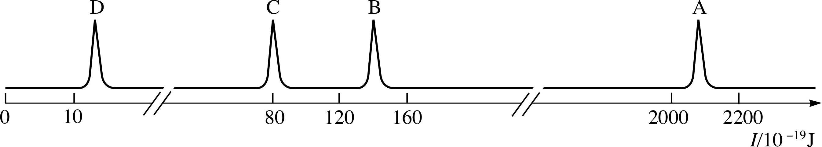
Figure 22 See Question E1.
Figure 22 shows the photoelectron spectrum of magnesium. Identify the electron subshells corresponding to each of the ionization energies and decide how many electrons are in each subshell (an atom of magnesium contains 12 electrons). Hence write down the electronic configuration of magnesium.
Answer E1
The peaks in the photoelectron spectrum (A, B, C, D) are the subshells s, 2s, 2p and 3s, respectively. The number of electrons in each subshell is: s (two), 2s (two), 2p (six) and 3s (two). The electronic configuration is therefore s2 2s2 2p6 3s2.
(Reread Subsections 2.2 and 2.3 if you had difficulty with this question.)
Question E2 (A5)
Write the electronic configurations for the elements oxygen and sulphur.
The atomic numbers are 8 and 16, respectively.
Answer E2
oxygen s2 2s2 2p4 sulphur s2 2s2 2p6 3s2 3p4
(Reread Subsections 3.1, 3.2 and 3.3 if you had difficulty with this question.)
Question E3 (A8)
Write the electronic configuration of nitrogen using the box representation.
The atomic number is 7.
Answer E3
The electronic configuration of nitrogen is represented by:
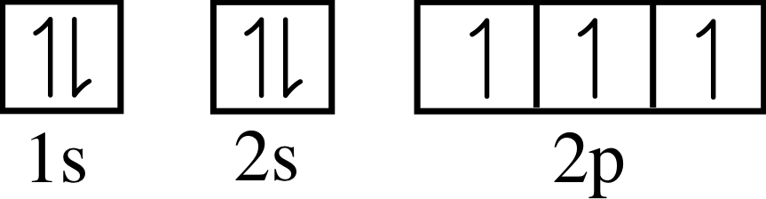
(Reread Subsection 3.3 if you had difficulty with this question.)
Question E4
(A3, A4, A6 and A7) State whether each of the following four statements about electron spin is true or false. In the cases in which you think the statement is false, give reasons for your answer.
(a) If a uniform magnetic field is used in an experiment that is otherwise similar to that of Stern and Gerlach, the beam would always be split into a number of components.
(b) Since the spin angular momentum quantum number of an electron is always 1/2, there are only two allowed orientations of the electron’s spin angular momentum vector S with respect to an arbitrary z–direction.
(c) Since the spin magnetic quantum number ms has two values, there are two possible values for the magnitude S of the spin angular momentum vector.
(d) The spin angular momentum quantum number of an electron is always s = 1/2, whether or not the electron is confined in an atom.
Answer E4
(a) False. The beam would not be split because a net magnetic force acts on the atomic ‘magnets’ (i.e. the atoms themselves) only when the magnetic field is non–uniform.
(b) True. The number of orientations is 2: ms = +1/2 and ms = −1/2.
(c) False. The magnitude of the spin angular momentum is given by $S^2 = s(s + 1)\hbar^2$. It does not depend on ms and the single value s = 1/2 gives $S = \dfrac{\sqrt{3\os}}{2}\hbar$.
(d) True. The spin of an electron is an intrinsic property of the electron whether or not it is in an atom.
(Reread Subsections 4.3 and 4.4 if you had difficulty with this question.)
Figure 20 The X–ray spectrum of molybdenum between λ = 0.02 nm and 0.22 nm shown for different acceleration voltages.
Question E5 (A6)
(a) Describe the physical process that gives rise to the emission of characteristic X–rays.
(b) What can be concluded from Figure 20 about the energy levels of molybdenum?
Estimate the energies by which these levels are separated.
Answer E5
(a) In one of the atoms in the target, the electron in one of the lowest energy levels is ejected by one of the electrons that are bombarding the target. (The bombarding electron, although deflected, continues on its way after this encounter.) An electron in a higher energy level makes a transition to the lower energy level vacancy, thereby replacing the ejected electron. During such a transition, a characteristic X–ray is emitted.
(b) A characteristic X–ray is emitted when an electron makes a transition between two energy levels separated by, typically, thousands of electronvolts. The wavelength of the X–ray and the spacing ∆E between the energy levels are related by the expression
λ = hc/∆E
From Figure 20, you can see that the wavelengths of two of molybdenum’s characteristic X–ray spectral lines are 0.063 nm and 0.072 nm.
For the first of these spectral lines:
E = [(6.6 × 10⁻³⁴ J s) × (3 × 10⁸ m s−1)]/(6.3 × 10−11 m) = 3.1 × 10⁻¹⁵ J = 20 keV
This calculation shows that two of molybdenum’s energy levels are separated by 20 keV.
By doing a similar calculation, you can show that the presence of the characteristic X–ray line of wavelength 0.072 nm in the molybdenum spectrum implies that another pair of molybdenum’s energy levels are separated by 17 keV.
(Reread Subsections 5.1 and 5.2 if you had difficulty with this question.)
Question E6 (A3 and A4)
How many electrons can be accommodated in the n = 3 shell of an atom?
What is the electronic configuration of a fully occupied n = 3 electron shell?
Answer E6
There are 2n2 = 18 electrons in a full n = 3 shell:
- two electrons in the l = 0 (s) subshell
- six electrons in the l = 1 (p) subshell in three degenerate (equal energy) quantum states with ml = +1, 0 and −1
- ten electrons in the l = 2 (d) subshell in five degenerate quantum states with ml = +2, +1, 0, −1 and −2.
The electronic configuration of the n = 3 shell is therefore 3s2 3p6 3d10.
(Reread Subsection 3.1 if you had difficulty with this question.)
Question E7 (A5, A6 and A7)
How would beams of the following atoms behave if passed through a Stern–Gerlach apparatus:
(a) neon (atomic number 10, chemical symbol Ne),
(b) sodium (atomic number 11, chemical symbol Na)?
Explain your answers.
Answer E7
(a) No effect; the ten electrons in a neon atom in its ground state fill the s, 2s and 2p shells: s2 2s2 2p6. All electron spins are paired, so there is no resultant magnetic effect.
(b) Sodium however has 11 electrons, so at least one of these must be unpaired. In fact only the electron in the 3s level is unpaired: s2 2s2 2p6 3s1. This electron has no orbital angular momentum; consequently the beam of sodium atoms splits into two in a non–uniform magnetic field, corresponding to the two spin states of the unpaired 3s electron. Therefore the sodium beam is split into two beams.
(Reread Subsection 4.3 if you had difficulty with this question.)
Study comment This is the final Exit test question. When you have completed the Exit test go back and try the Subsection 1.2Fast track questions if you have not already done so.
If you have completed both the Fast track questions and the Exit test, then you have finished the module and may leave it here.
Study comment Having seen the Fast track questions you may feel that it would be wiser to follow the normal route through the module and to proceed directly to the following Ready to study? Subsection.
Alternatively, you may still be sufficiently comfortable with the material covered by the module to proceed directly to the Section 5Closing items.