PHYS 6.3: Optical elements: prisms, lenses and spherical mirrors |
PPLATO @ | |||||
PPLATO / FLAP (Flexible Learning Approach To Physics) |
||||||
|
1 Opening items
1.1 Module introduction
You will probably be familiar with the action of a prism in splitting white light into the colours of the rainbow, or of a simple magnifying lens, or of the curved reflectors used in vanity mirrors, shaving mirrors and driving mirrors. This module describes these optical elements and introduces you to the equations which govern their operation and which can be used in their design. The operation of all these optical elements depends on the known behaviour of light rays when reflected from mirrors or refracted at the boundary between two transparent optical media. The magnifying glass is just one application of a thin lens and the mirrors listed above are examples of spherical mirrors. An understanding of the action of these simple optical elements opens the way to an understanding of more complex instruments, such as telescopes, microscopes, camera lenses and projection systems, which are discussed in other FLAP modules.
Section 2 describes refraction by a prism, using Snell’s law, and shows how prisms can be used to produce dispersion and total internal reflection. Section 3 describes refraction at a single spherical surface using a Cartesian sign convention and introduces the conjugate equations for refraction at this surface and for refraction by a thin lens. The focal length for a thin lens is introduced and the lens maker’s equation and the thin lens equation are derived. Convex and concave lens behaviour is then discussed using this formula, ray diagrams and principal rays. The transverse magnification and optical power of a lens are described, as is the process of image formation in a two–lens system.
In Section 4 we extend these ideas to convex and concave spherical mirrors using the same Cartesian sign convention. The spherical mirror equation is derived, and this is used with ray diagrams to discuss the operation and transverse magnification of spherical mirrors.
It is interesting to note that although the fundamental principles of reflection and refraction were discovered nearly three hundred years ago, the subject has seen something of a renaissance recently with the advent of fast computer systems; complex lens systems can now be designed quickly. This has led to a resurgence of interest in optics in general and in particular to the use of optical components in advanced technology and physics research. However, this creates plenty of scope for gettings things wrong on an impressive scale, as was shown in the case of the Hubble space telescope. This was launched in 1990 and had a wrongly configured main mirror. The problem has now been corrected with the help of an additional optical system, installed in orbit by NASA astronauts.
Study comment Having read the introduction you may feel that you are already familiar with the material covered by this module and that you do not need to study it. If so, try the following Fast track questions. If not, proceed directly to the Subsection 1.3Ready to study? Subsection.
1.2 Fast track questions
Study comment Can you answer the following Fast track questions? If you answer the questions successfully you need only glance through the module before looking at the Subsection 5.1Module summary and the Subsection 5.2Achievements. If you are sure that you can meet each of these achievements, try the Subsection 5.3Exit test. If you have difficulty with only one or two of the questions you should follow the guidance given in the answers and read the relevant parts of the module. However, if you have difficulty with more than two of the Exit questions you are strongly advised to study the whole module.
Question F1
Sketch a ray diagram to show how a thin convex lens can be used as a magnifying glass. Use your diagram to find the magnification if the object distance is 10 cm and the image distance is 25 cm?
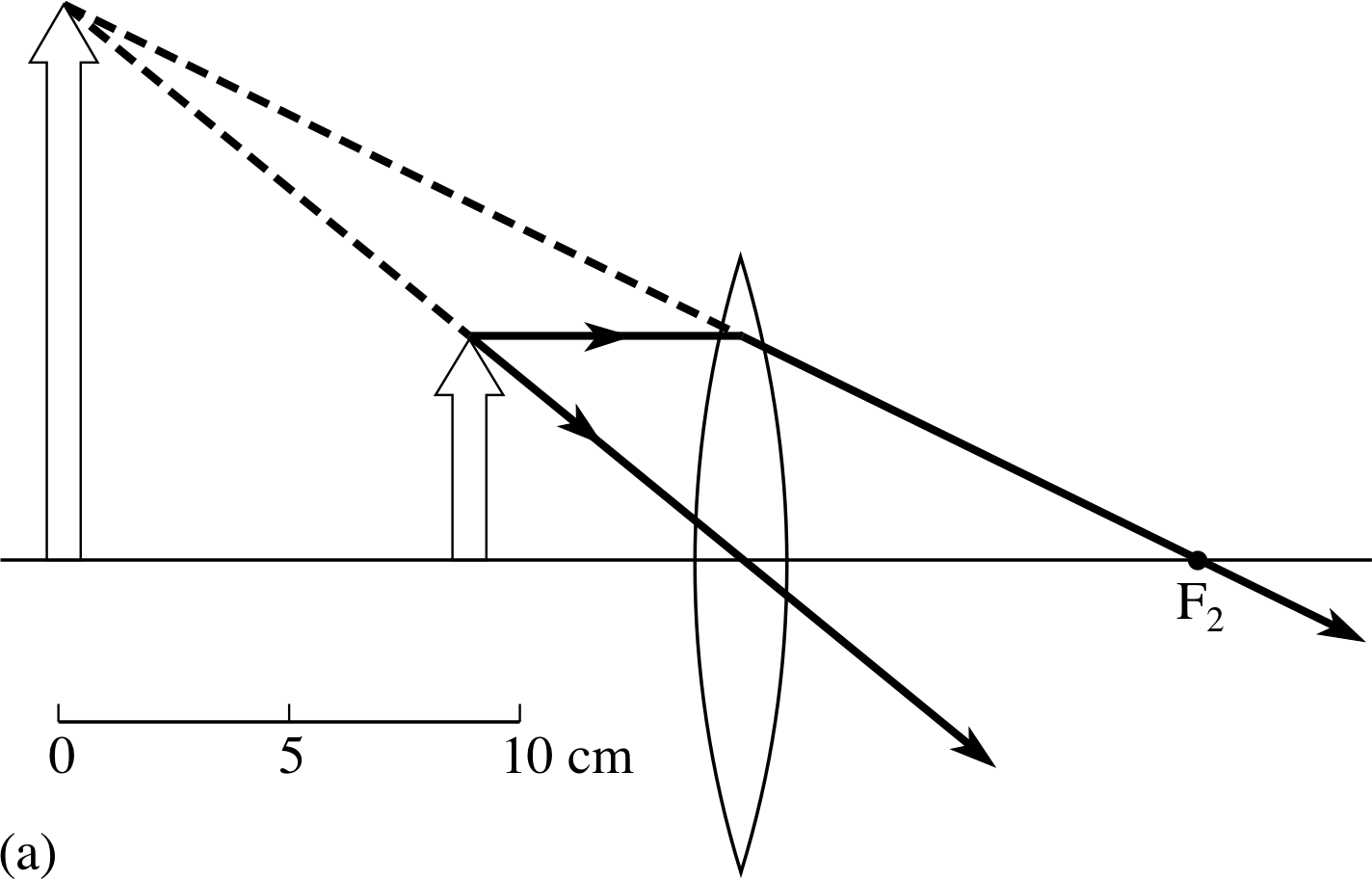
Figure 27a See Answer T5. A convex lens used as a magnifying glass.
Answer F1
Figure 27a (in the answer to Question T5) shows a diagram similar to that required, but with different dimensions. The object is between the first focus and the lens. The image is erect and virtual. The lateral magnification m = υ/u, so m = (−25 cm)/(−10 cm) = +2.5. (υ is the image distance, u is the object distance and the Cartesian sign convention has been used.)
Question F2
An extended object is placed 25 cm from a converging lens of focal length 10 cm. Use the thin lens equation to calculate the position of the image. Is the image real or virtual? What is the magnification? Draw a ray diagram to show the location of the image.
Answer F2
Use the thin lens equation (Equation 12),
The thin lens equation (Cartesian sign convention) $\dfrac{1}{\upsilon} - \dfrac{1}{u} = \dfrac{1}{f}$(Eqn 12)
with u = −25 cm, f = +10 cm, so that:
1/υ = (1/10 cm) + (−1/25 cm) = (5−2)/(50 cm) = 3/(50 cm) and υ = +50 cm/3 = +16.7 cm.
The image is real and inverted with a magnification m = υ/u = 16.7 cm/25 cm = 0.67.
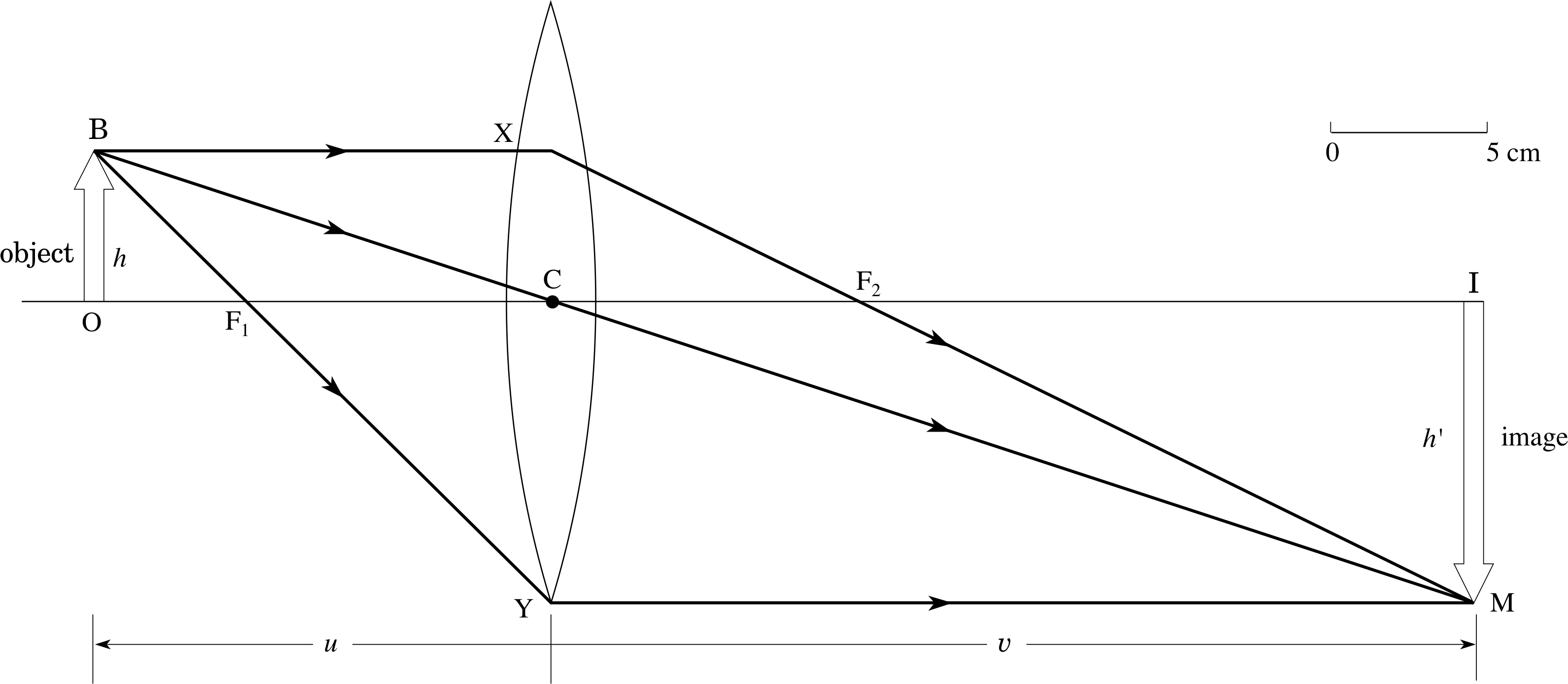
Figure 19 Ray diagram for a convex lens with f = 10 cm and u = −15 cm. Note that the zero on the scale bar does not correspond to the origin of Cartesian coordinates which is at C.
Your sketch should resemble Figure 19 but with the object further from the lens, and the image closer and smaller than the object.
Question F3
A concave mirror has focal length of 10 cm. Draw a ray diagram to find the image position of an extended object placed 15 cm from the mirror. Confirm your result by direct calculation.
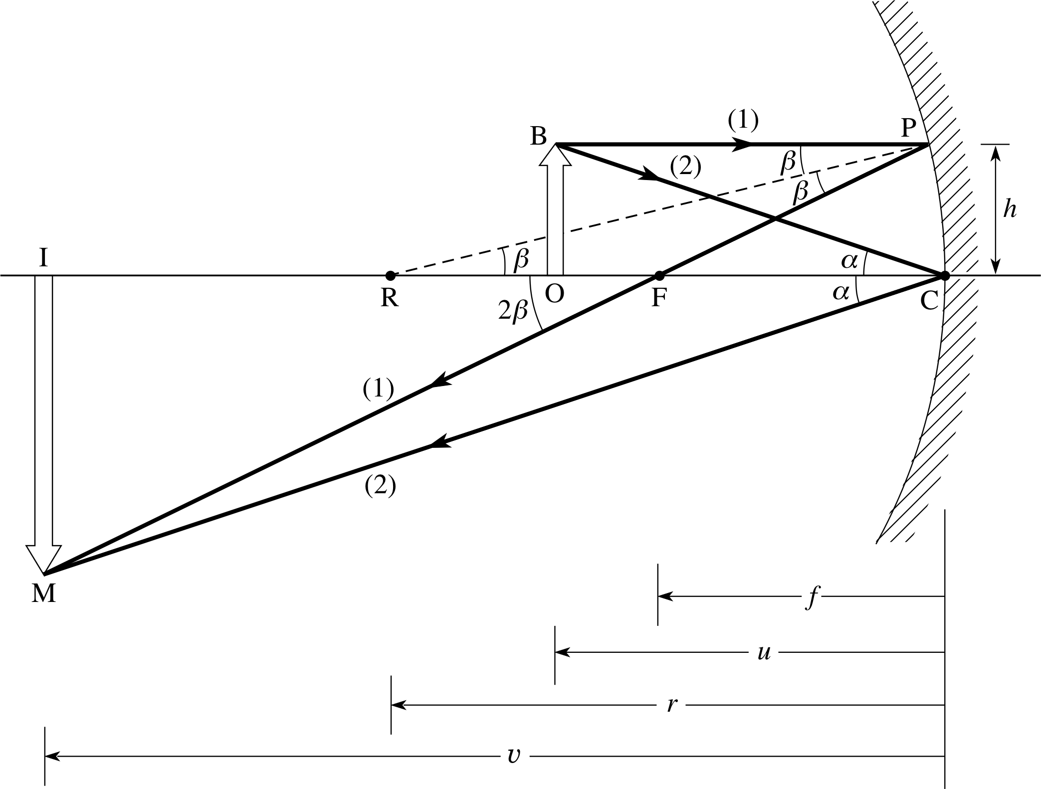
Figure 24 A spherical concave mirror forming a real inverted image of an extended object.
Answer F3
The ray diagram is similar to Figure 24. Use the formula 1/u + 1/υ = 1/f with u = −15 cm and f = −10 cm.
Then 1/υ = (1/−10 cm) − (1/−15 cm) = (−3 + 2)/(30 cm) = −1/(30 cm), and υ = −30 cm.
The image is real, inverted and 30 cm in front of the mirror.
1.3 Ready to study?
Study comment Throughout this module we will use geometrical optics for the propagation of light (i.e. the ray approximation, neglecting any diffraction effects). We will use the law of reflection of light at plane mirrors, and Snell’s law for the refraction of light at an interface between two transparent materials of different refractive index. We will assume and use total internal reflection and the relationship between refractive index and the speed of light in the material.
Mathematical requirements are mainly elementary trigonometry and algebra, the geometry of triangles and especially the approximationsmall angle approximations for sine, cosine and tangent. You should also be familiar with the use of Cartesian coordinates and the solution of quadratic equations.
If you are uncertain about any of these terms you can review them now by referring to the Glossary which will indicate where in FLAP they are developed.
The following Ready to study questions will allow you to establish whether you need to review some of the topics before embarking on this module.
Question R1
State the law of reflection for light rays at a plane mirror.
Answer R1
(i) The incident ray, the reflected ray and the normal at the reflection point all lie in the same plane.
(ii) The angle of the incident ray to the normal equals the angle of the reflected ray to the normal.
Question R2
A light ray passes from air into glass with refractive index 1.50. The angle of incidence is 15°, calculate the angle of refraction and the speed of the light inside the glass. (The speed of light in a vacuum is 3.0 × 10⁸ m s−1).
Answer R2
Snell’s law says: μair sin θair = μglass sin θglass. The ray is refracted towards the normal since μ2 > μ2 ≈ 1.00. We have:
θglass = arcsin (sin θair /μglass) = arcsin(0. 259/1.50) = arcsin(0.173) = 9.9°
The refractive index μglass = c/υ, where υ is the speed of light in the material and c is the speed of light in a vacuum:
υ = 3.0 × 10⁸ m s−1/1.5 = 2.0 × 10⁸ m s−2
Question R3
Show by calculation that the error is less than about 1% if we assume that tan θ = θ and sin θ = θ for angles smaller than 0.17 rad (about 10°).
Answer R3
At 10°, tan θ = 0.1763 and θ = 10π/180 = 0.1745 radians.
The percentage error is: (0.0018/0.1763) × 100% = 1%.
At 10°, sin θ = 0.1736 and the percentage error is: (0.0009/0.1736) × 100% = 0.5%.
The approximation improves as θ gets smaller.
2 Refraction by a prism
2.1 A parallel–sided glass block
Figure 1 The refraction of a ray of light through a parallel–sided glass block.
We will start our discussion of how light is refracted by a glass prism by recalling what happens to light as it travels through a block of glass as shown in Figure 1.
When a ray of light of a single wavelength (i.e. a monochromatic ray) enters the glass (an optically dense medium) from the air (an optically rare medium), it is refracted towards the normal to the boundary according to Snell’s law of refraction: i
μ1 sin θ1 = μ2 sin θ2(1)
where μ1 and μ2 are the refractive indices of air and glass, and θ1 and θ2 are the angles of incidence and refraction at the boundary. The refractive index of air is about 1.0003, which we approximate to 1, so that Equation 1 becomes:
sin θ1 = μ2 sin θ2(2)
After the ray has crossed the block, its angle of incidence on the second boundary is θ3, and it emerges, refracted away from the normal, at θ4. However, since the block is parallel-sided, θ3 = θ2 so that:
μ2 sin θ2 = μ2 sin θ3 = sin θ4(3)
Comparing Equations 2 and 3 shows us that θ1 = θ4, so the ray emerges in the same direction as it entered, but has suffered a lateral shift.
✦ Is it true to say that the ray always suffers a lateral shift here?
✧ No, there is no lateral shift if the ray is normal to the block faces, i.e. travelling perpendicular to the surfaces.
2.2 Refraction by a prism
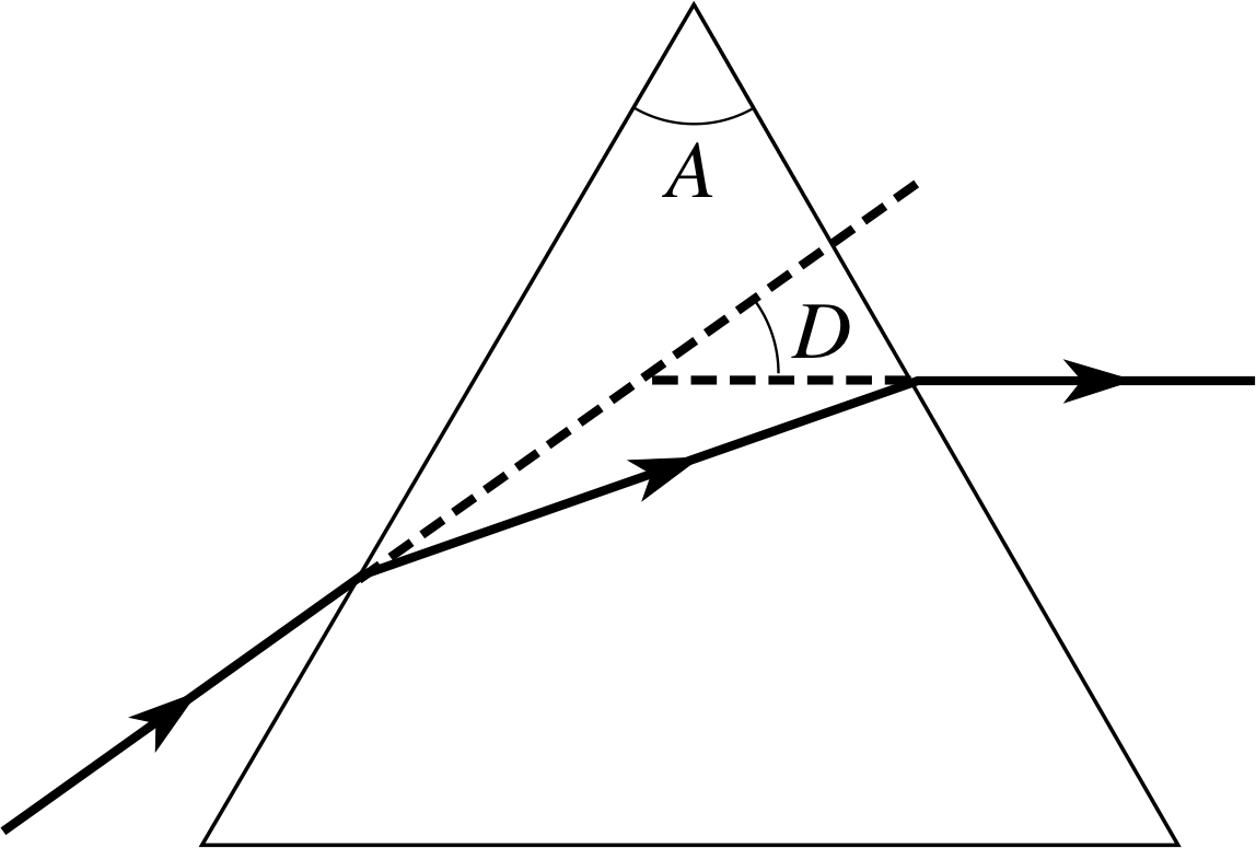
Figure 2 Refraction by a prism, showing the prism angle A and the angle D by which the ray is deviated.
When the second face of the block is not parallel to the first, the path of a monochromatic ray will in general be like that through the prism of Figure 2, and will no longer have the symmetry of Figure 1. The ray leaving the prism will not be parallel to the ray entering the prism, as it will have been deviated by it, having turned through the angle of deviation D.
However, there is a situation in which a different symmetry is present; this occurs when the ray in the glass makes equal angles with the two prism faces, as in Figure 3. This geometry may be shown to have the important consequence that it makes the angle of deviation a minimum for any given wavelength. A relationship between this angle of minimum deviation and the prism angle A, which is the angle between the refracting faces of the prism, can be obtained as follows. i
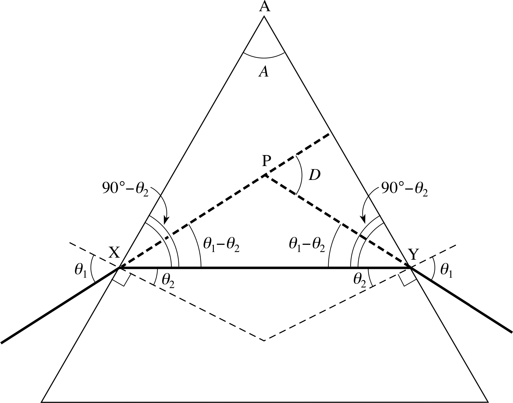
Figure 3 Refraction of a ray whose path makes equal angles with the two refracting faces of the prism. This is a ray of minimum deviation.
For triangle PXY we have Dmin = 2(θ1 − θ2), and in triangle AXY, A + 2(90° − θ2) = 180°, so that A = 2θ2. Combining these equations gives the minimum deviation Dmin = 2θ1 − A. Then, using Snell’s law,
$\mu = \dfrac{\sin\theta_1}{\sin\theta_2} = \dfrac{\sin\left[\frac12 (D_{\rm min}+A)\right]}{\sin\left(\frac12 A\right)}$(4)
This equation can be rearranged to give an expression for Dmin:
Dmin = 2 arcsin[μ sin(A/2)] − A(5)
2.3 Prisms in optical instruments
There are two principal applications of prisms in optical instruments; they are dealt with in detail elsewhere in FLAP and so we will discuss them here only very briefly. They involve dispersion and total internal reflection – topics which are themselves introduced more fully elsewhere in FLAP.
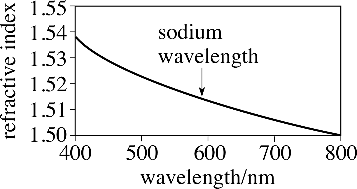
Figure 4 The wavelength dependence of the refractive index of borosilicate crown glass. If a single value is quoted for a refractive index, it is usually at the sodium wavelength of 589.3 nm.
Dispersion is the splitting up of a beam of light of mixed wavelengths into its constituent wavelengths. The reason why a prism can perform this task is that the refractive index μ varies with the wavelength of the light being refracted, as is shown for a common type of borosilicate glass in Figure 4. Now referring to Equation 2,
sin θ1 = μ2 sin θ2(2)
we see that for incidence at a given angle θ1, the angle of refraction θ2 depends on the refractive index μ2, which in turn depends on the wavelength. Tables which summarize the physical properties of materials often quote a single value of μ for a particular type of glass; this single value is then usually for sodium light, with a mean wavelength of 589.3 nm. i
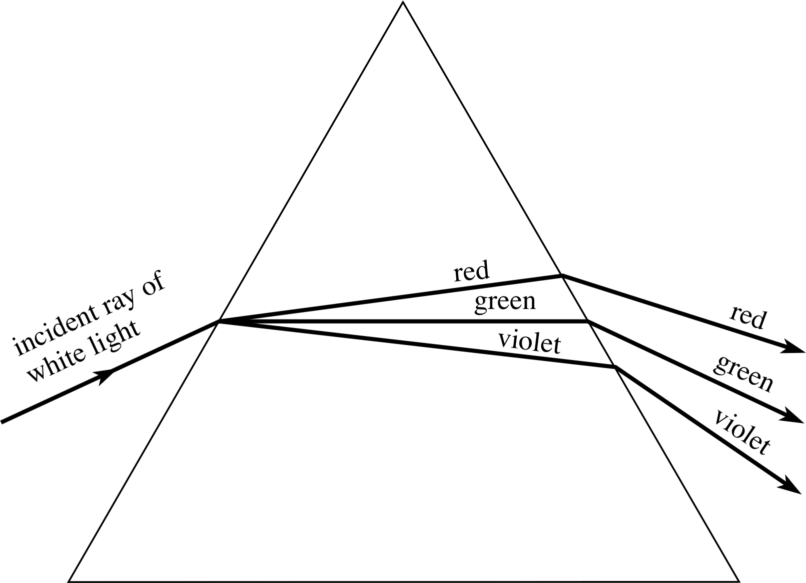
Figure 5 The dispersion of white light by a prism. Only three of the spectrum colours are shown and the dispersion is greatly exaggerated. Note that the red light suffers less deviation than the green. This does not conflict with the fact the symmetric path is the path of minimum deviation for any given wavelength. The red light would suffer even less deviation if it was in the symmetric position.
If we have a beam of light which contains a range of different wavelengths (e.g. white light) incident at angle θ1 then there will be a range of refracted angles θ2, with shorter wavelengths (e.g. violet) being refracted or deviated through larger angles than the longer wavelengths (e.g. red). If the surface where this refraction occurs is the first surface of a prism, then further dispersion of the different constituent wavelengths takes place at the second surface, as shown in Figure 5 (in which the angles of dispersion are exaggerated). A prism being used for dispersion is usually orientated so that it is in a position of minimum deviation for the middle of the range of wavelengths present in the beam. This arrangement produces the minimum dispersion, but it also causes the graph of angle of deviation against wavelength to be nearly linear, i.e. it corresponds to linear dispersion.
| Colour | Wavelength /nm | μ | Dmin/° |
|---|---|---|---|
| blue | 450 | 1.519 | |
| green | 550 | 1.515 | |
| yellow | 590 | 1.508 | |
| red | 650 | 1.502 |
Question T1
Calculate the angle of minimum deviation at various wavelengths for a 60° prism made of crown glass and hence complete Table 1.
Answer T1
The apex angle A of the prism is 60°. Using Equation 5 for Dmin:
Dmin = 2 arcsin[μ sin(A/2)] − A(Eqn 5)
blue light:Dmin = 2 × 49.42° − 60° = 38.84°
green light:Dmin = 2 × 49.24° − 60° = 38.49°
yellow light:Dmin = 2 × 48.94° − 60° = 37.88°
red light:Dmin = 2 × 48.68° − 60° = 37.35°
The second important application of prisms is their use as reflectors. If we restrict our discussion to a single wavelength, then we see that as the angle of incidence of a light ray on the second face of a prism is increased, an angle will be reached when the refracted ray travels along the surface of the prism (Figure 6a) corresponding to an angle of refraction θ2 = 90°. The angle of incidence within the glass at which this happens is the critical angle θc and, if this angle is exceeded, then total internal reflection occurs (Figure 6b).
The type of prism usually employed for its ability to produce such internal reflections is the 45°/90°/45° prism, which may be used in the two orientations shown in Figure 7.
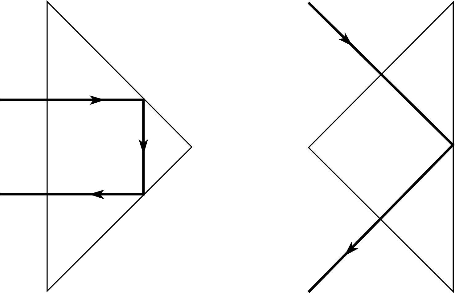
Figure 7 Two ways in which a 45°/90°/45° prism may be used as a reflector.
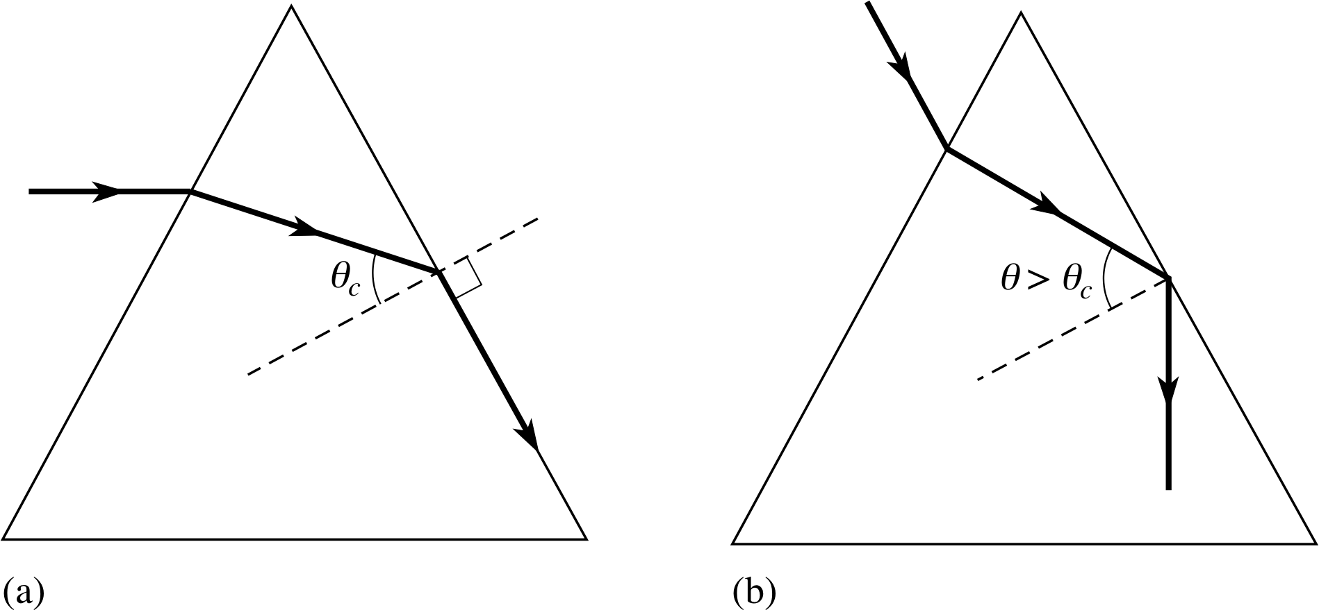
Figure 6 (a) A ray making a critical angle of incidence θc to the second face of the prism; (b) a ray which is totally reflected, having θ > θc.
3 Refraction at a single spherical boundary
Our objective in this section of the module is to derive and apply equations governing the passage of rays of light through lenses, which are usually discs of glass or other transparent material, with one or both surfaces curved symmetrically about the optical axis of the lens. The optical axis is the line drawn normal to the disc and through its centre. We restrict our discussion to lenses having surfaces of a constant radius of curvature and therefore described as spherical lenses, and also to thin lenses, where the maximum distance between the faces is very small compared with the radius of curvature of either face. We include the possibility of one of the surfaces being flat, i.e. of having an infinite radius of curvature.
The first stage of our discussion is to establish the conjugate equation which describes the refraction of light at a single spherical surface, by which we mean the spherical boundary between regions of uniform refractive index μ and μ′. This is a system which has only limited practical application, although as we shall see, it does have important image–forming properties. However, when we have obtained an equation which describes what happens to light at a single spherical surface, then we can apply it again at a second spherical surface: two such surfaces in close succession, with appropriate changes of index, are what we mean by a lens.
3.1 The conjugate equation for a single spherical surface
We start by considering the refraction of a monochromatic light ray OA which leaves a point source of light O in Figure 8, situated on the optical axis at a distance l to the left of the vertex_of_a_lensvertex or pole_of_a_lenspole C of the curved boundary (which is the point where the optical axis intersects that boundary).
Figure 8 Refraction at a spherical boundary of a ray of light from a point source.
We will assume that the refractive index μ′ of the medium to the right of the boundary is greater than the index μ to the left. The ray is therefore refracted towards the normal to the boundary, and crosses the optical axis at O′, a distance l′ from C. Snell’s law of refraction when applied at A gives:
μ sin θ = μ′ sin θ′(6)
where θ and θ′ are the angles of incidence and refraction measured with respect to the normal AR to the boundary at A.
We now introduce a most important restriction to our discussion and assume that:
all light rays, and normals to the boundary surface are either parallel to the optical axis or are at very small angles (i.e. not more than 10°) to it. This is known as the paraxial approximation, and rays which conform to it are called paraxial rays.
In any system subject to this approximation, we may write the sine or tangent of the angles made by any ray to the axis or to any other ray or to any radius of curvature of the boundary, as equal to the angles themselves, measured in radians.
If we now apply the paraxial approximation to Equation 6 we obtain:
μθ = μ′θ′
From the triangles in Figure 8 we have:
θ = α + β and β = θ′ + γ
so that μ (α + β) = μ′ (β − γ)
We now replace the angles in this equation by their tangents, writing
α = tan α = h/l, β = tan β = h/r, γ = tan γ = h/l′
where h is the distance of A from the optical axis and we have made the approximation that C is directly below A.
Then,$\mu\left(\dfrac hl + \dfrac hr \right) = \mu'\left(\dfrac hr - \dfrac{h}{l'}\right)$
Dividing by h and rearranging then gives:
$\dfrac{\mu}{l} + \dfrac{\mu'}{l'} = \dfrac{\mu'-\mu}{r}$(7)
Equation 7 allows us to calculate the distance l′ from the boundary, of the point where the refracted ray AO′ crosses the optical axis. As explained below, points O and O′ are examples of an object and an image in an optical system; any light ray originating from O arrives at O′. An important property of Equation 7 is that it does not contain h. Thus all rays from O are refracted so as to pass through O′ (as in Figure 8), no matter how far from the optical axis they cross the boundary, provided they may be regarded as paraxial rays. O′ is then said to be the point image of the point object O. Moreover, if it were possible to place a screen at O′, then the image would be displayed on the screen and such a ‘captured’ image, where the rays converge and pass through a point, is called a real image. Note that the ray which coincides with the optical axis remains undeviated because it is at normal incidence to the boundary. i
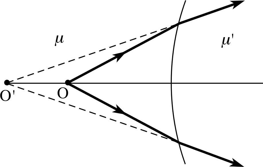
Figure 9 A point object projections of rays are shown by dashed lines, indicating that light does not travel close to a curved boundary. along such paths.
A point object placed to the left of a curved boundary, as in Figure 8, does not always result in a real point image being formed to the right of the boundary. If the object is brought closer to the same boundary as in Figure 9, then again provided that μ′ > μ, rays from the object to the boundary will be refracted towards the normal but will not converge to a point on the optical axis – instead they appear to diverge from a point to the left of the object position. Such a point is called a virtual image. It cannot be captured on a screen as rays do not actually pass through it but only appear to have come from that point when viewed from the right of the boundary. You will notice that a convention has been introduced in Figure 9 whereby the paths followed by rays of light are shown by thick lines; similar analysis to that applied to Figure 8 leads to an equation containing identical terms to those in Equation 7, but with some differences in the signs of the terms. We will examine those differences shortly.
The boundary surfaces which we have been examining bulge towards the object position and, when seen from that side, are called convex surfaces. We can also examine the refracting properties of spherical boundaries which are hollow when seen from the left; these are called concave surfaces.
Question T2
With similar reasoning to that used to establish Equation 7,
$\dfrac{\mu}{l} + \dfrac{\mu'}{l'} = \dfrac{\mu'-\mu}{r}$(Eqn 7)
show that the conjugate equation connecting object position and the apparent origin of the diverging rays for the concave boundary system shown in Figure 10 is: $\dfrac{\mu'}{l'} - \dfrac{\mu}{l} = \dfrac{\mu'-\mu}{r}$

Figure 10 The point image of a point object formed by a concave boundary surface (see Question T2).
Answer T2
In the paraxial approximation, μ = μ′θ′
From the triangles of Figure 10 we have:
θ = β − α and θ′ = β − γ, so that μ (β − α) = μ′(β − γ)
Replacing angles by their tangents then gives:
β = tan β = h/r, α = tan α = h/l and γ = tan γ = h/l′
so$\mu\left(\dfrac hr-\dfrac hl\right) = \mu'\left(\dfrac hr-\dfrac{h}{l'}\right)$
and$-\dfrac{\mu}{l} + \dfrac{\mu'}{l'} = \dfrac{\mu'-\mu}{r}$
This differs from Equation 7,
$\dfrac{\mu}{l} + \dfrac{\mu'}{l'} = \dfrac{\mu'-\mu}{r}$(Eqn 7)
in the sign of the first term.
Another situation which could be analysed has the object closer to the concave surface than in Question T2. If we chose, we could also analyse four sets of object and image positions when the second medium had a lower refractive index than the first. However, we would find that the equations resulting from all eight possibilities differed only in the signs of the terms. We can surmise from this that if the different systems were specified more completely, then they could all be described by the same equation. This is in fact the case, and the additional information required is the location of object, image and centre of curvature positions with respect to the boundary vertex.
What we have used so far are the distances of O, O′ and R from C, when we should have used their displacements. This is easily rectified by introducing a sign convention which will enable us to attach a sign to these distances and which, in effect, converts them into displacements (although we will continue to call them distances because this is the normal practice in optics). There are several possible conventions and we will adopt the one most commonly used, which is the Cartesian sign convention. i Although it is being introduced here for refraction at a single curved surface, it will be applied to lenses in Subsection 3.2 and to mirrors in Section 4.
It is defined as follows:
The Cartesian sign convention
- 1
-
The origin of a Cartesian system of coordinates is located at the vertex of the curved boundary or mirror, or at the centre of a thin lens, with the z–axis directed along the optical axis from left to right.
- 2
-
Object, image and centre of curvature distances (really, displacements) are defined to be the z– coordinates of the (x, y) planes which contain them. Distances of points or planes to the right of the vertex (or lens centre) therefore are given positive signs and those to the left, negative signs.
- 3
-
Light sources or real objects will be placed diagrammatically to the left of the first optical surface, thus the initial paths of light rays travel from left to right in the positive z–direction, which means that the object distance is taken as negative.
Figure 8 Refraction at a spherical boundary of a ray of light from a point source.
We can now see what effect this convention has on Equation 7,
$\dfrac{\mu}{l} + \dfrac{\mu'}{l'} = \dfrac{\mu'-\mu}{r}$(Eqn 7)
In Figure 8, the object O is to the left of C so l becomes −l; the image O′ is to the right, so l′ retains its positive sign, as does r, since R is also to the right of C.
Now see for yourself what changes this convention makes to the result obtained in Question T2.
Question T3
Modify the equation given in Question T2,
$\dfrac{\mu'}{l'} - \dfrac{\mu}{l} = \dfrac{\mu'-\mu}{r}$
(and illustrated in Figure 10) according to the Cartesian sign convention.
Answer T3
Figure 10 The point image of a point object formed by a concave boundary surface (see Question T2).
Referring to Figure 10 we see that O, O′ and R all lie to the left of the origin at C so that l, l′ and r must all be made negative. With these changes, the equation which forms the answer to Question T2 is unchanged.
You should have obtained exactly the same result as the modified Equation 7 (see Answer T2) and it would also be obtained for the other six configurations. This new form of the equation, shown below, is called the conjugate equation for a single spherical surface; it is an equation which links together the object and image distances and the radius of curvature of the spherical surface at which refraction occurs.
The conjugate equation for a single spherical surface (Cartesian version):
$\dfrac{\mu'}{l'} - \dfrac{\mu}{l} = \dfrac{\mu'-\mu}{r}$(8)
To interpret this in the general case (convex or concave), with light moving from left to right, remember that μ is the refractive index to the left of the interface, μ′ is the refractive index to the right of the interface, l is the object distance, l′ is the image distance and r is the radius of curvature. The signs of l, l′ and r are determined by the Cartesian sign convention.
Even though we have incorporated the sign convention into Equation 8, when it is used for calculation, it is still necessary to allot signs to distances according to the sign convention before they are entered into the equation. Object and image points linked by the conjugate equation are called conjugate points, and planes perpendicular to the optical axis containing conjugate points are conjugate planes.
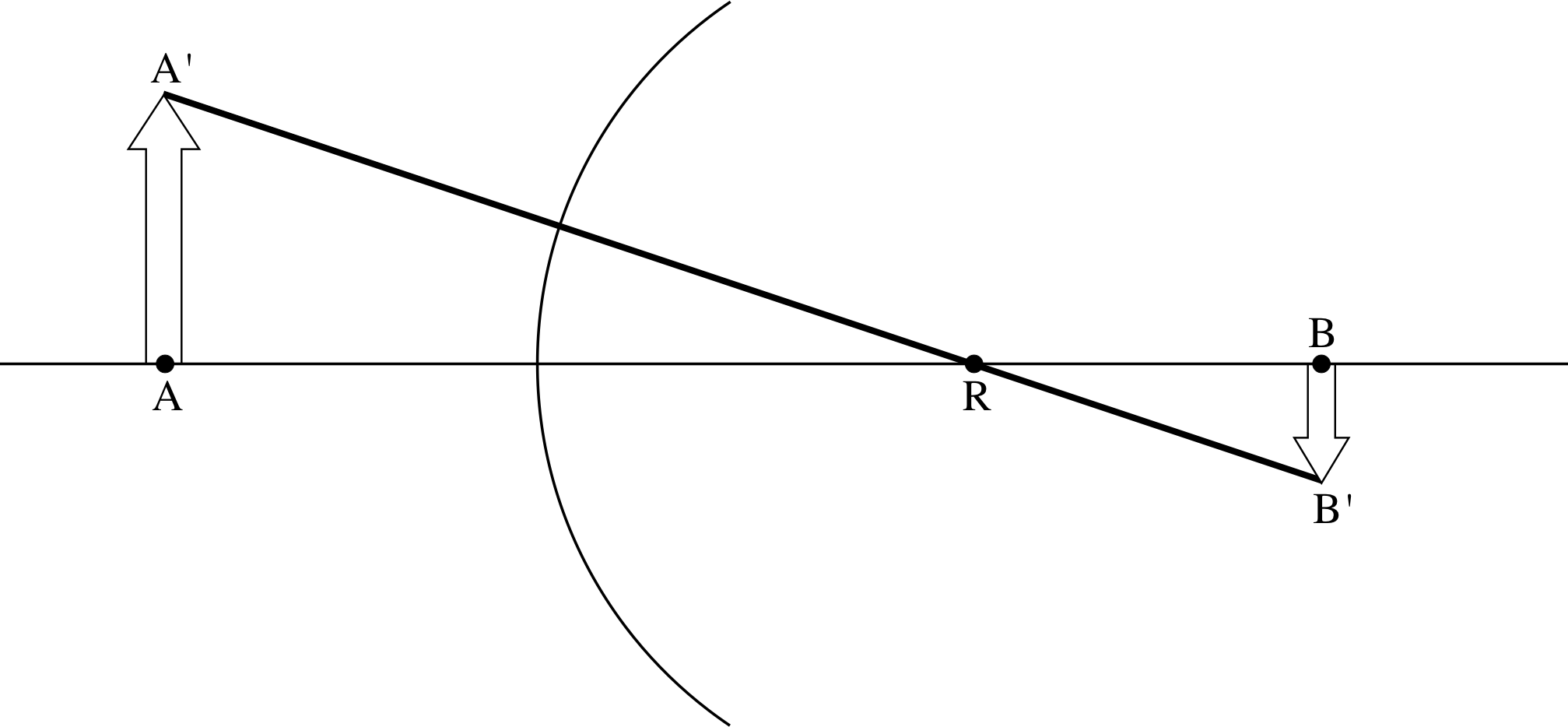
Figure 11 The extended image of an extended object.
We can extend our discussion of point objects to include objects of finite size by regarding a finite object as a continuous succession of point objects. For example, consider the image of the line object AA′ which is perpendicular to the optical axis in Figure 11. We will assume that the end A is imaged at B by the spherical surface with centre of curvature at R. The line joining the end A′ to R may be regarded as another optical axis and, within the paraxial approximation, an image of A′ will be formed at B′. If AA′ and BB′ are small, they may be assumed to be perpendicular to the original optical axis, and BB′ is then the extended image of the extended object AA′.
3.2 Refraction by a thin convex lens
When confronted with a compound system (i.e. more than one optical component), we can apply Equation 8,
$\dfrac{\mu'}{l'} - \dfrac{\mu}{l} = \dfrac{\mu'-\mu}{r}$(Eqn 8)
to each component in turn, treating the image produced by one lens as an object for the next one along. If we follow this procedure, using a consistent convention of signs throughout, then the image for the final component will be the image for the entire system.
With this in mind, we can now consider the refraction produced by two spherical surfaces with radii of r1 and r2, respectively, with the second surface a distance t from the first, along the common optical axis. These surfaces form a spherical lens, which has a refractive index μ and is surrounded by air with a refractive index of 1. Figure 12 shows such a lens, in this case a biconvex lens, since it has both faces convex as seen from the outside. Often a biconvex lens is simply called a convex lens.
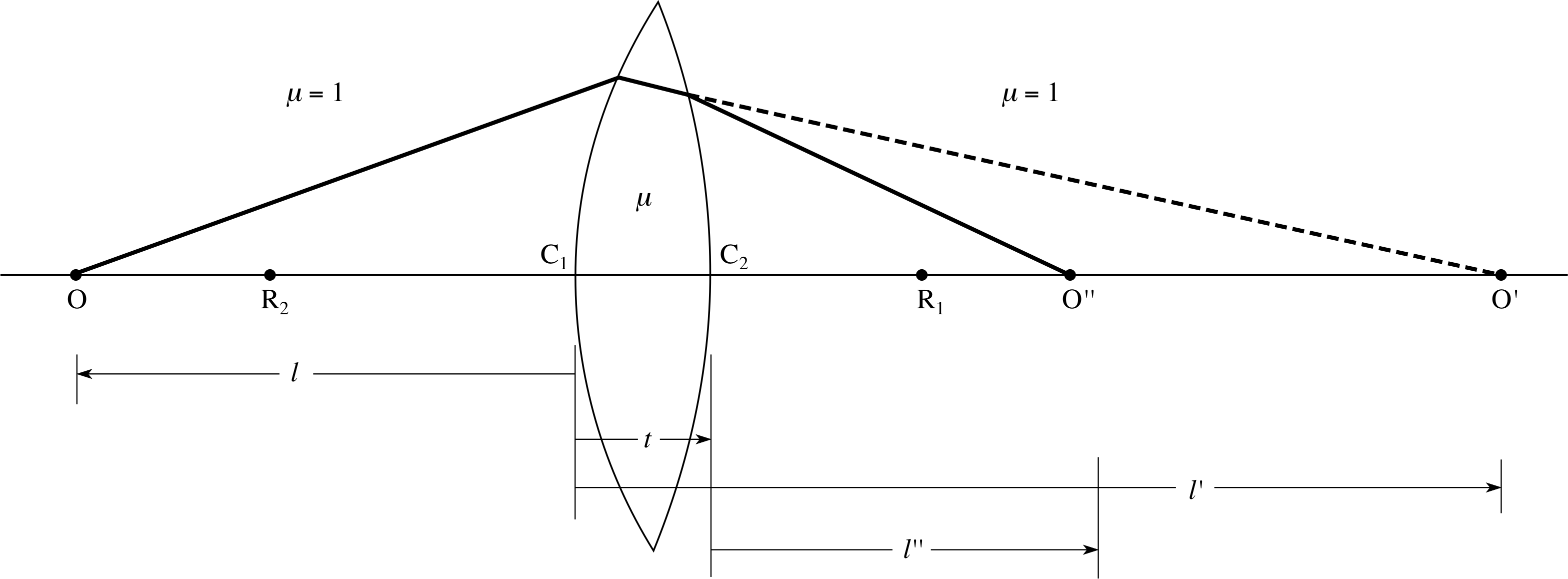
Figure 12 A convex lens forms a point image of a point object.
An axial point object O, is at a distance l from the vertex C1 of the first surface, which, by itself would form an image O′ at a distance l′ from C1. Equation 8 now relates object and image distances for this first (left-hand) surface:
$\dfrac{\mu}{l'} - \dfrac{1}{l} = \dfrac{\mu-1}{r_1}$ i
The image O′ now acts as an object for the second surface, being at a distance (l′ − t) from it, where t is the lens thickness. i The second surface produces an image O′′ of O′ at a distance l′′ from the vertex C2. Applying Equation 8 a second time gives:
$\dfrac{1}{l''} - \dfrac{\mu}{l'-t} = \dfrac{1-\mu}{r_2}$ i
We see from these two equations that there is no simple relationship between object and image distances for a finite value of t. However, simplification follows if the thickness t is much less than the object and image distances and each of the radii of curvature and can therefore be neglected; this is our thin lens approximation. Putting t = 0, and adding the last two equations gives: i
$\dfrac{1}{l''} - \dfrac{1}{l} = (\mu-1)\left(\dfrac{1}{r_1}-\dfrac{1}{r_2}\right)$(9)
We now make a change in the symbols used for object and image distances to accord with common practice and write the object distance l = u and the final image distance l′′ = υ. We then obtain the conjugate equation for a thin lens, relating object and image distances for a thin lens to the radii of curvature of its surfaces.
The conjugate equation for a thin lens
$\dfrac{1}{\upsilon} - \dfrac{1}{u} = (\mu-1)\left(\dfrac{1}{r_1}-\dfrac{1}{r_2}\right)$(10)
Remember that according to the Cartesian sign convention any of the quantities u, υ, r1 and r2 may be negative in this formula.
3.3 Focal points of a thin convex lens
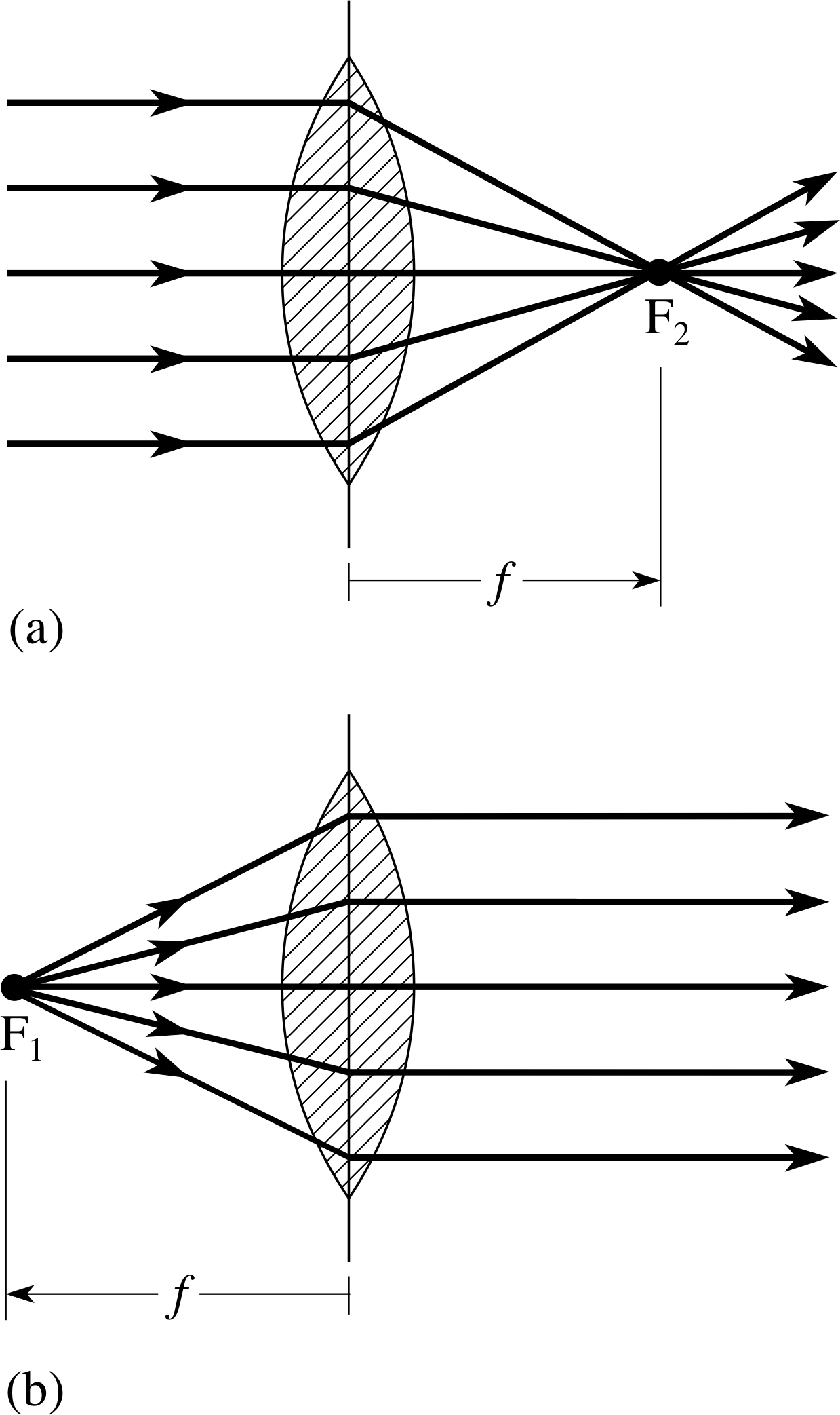
Figure 13 (a) Parallel rays from an object at infinity are brought to a focus at the second focal point, F2. (b) Paraxial rays diverging from a point object at the first focal point, F1, are made parallel by the lens. Note that for a thin lens, F1 and F2 are at equal distances from the centre of the lens, irrespective of the values of r1 and r2.
Now let us consider what happens when the object is moved further and further away from the lens, so that u is large compared to r1 and r2. We can take the limit as | u | → ∞ and 1/| u | → 0. i In this limit, all rays from the object which are incident on the lens will be parallel to the optical axis and will be refracted by the lens through a single image point on the axis, as shown in Figure 13a. This image point F2 is called the image focus or second focus or second focal point of the lens and it is situated at a distance f from the lens. The distance from the centre of the lens to F2 is called the focal length f of the lens and is the parameter by which the focusing property of the lens is quantified.
The focal length of a convex lens is the distance from the centre of the lens at which parallel rays from an object at infinity are brought to a focus.
This formal definition of focal length provides the basis of a simple method by which the focal length of a convex lens may be found. If the image of a distant object, such as a far window, tree, or house is focused on to a screen, then the distance from the lens centre to the screen will be slightly greater than the focal length. The further the object is from the lens, the closer the image distance will be to the focal length.
Equation 11 shows an expression for f obtained by putting 1/u = 0 in Equation 10,
$\dfrac{1}{\upsilon} - \dfrac{1}{u} = (\mu-1)\left(\dfrac{1}{r_1}-\dfrac{1}{r_2}\right)$(Eqn 10)
This is called the lens maker’s equation because it relates the surface radii required to produce a lens of a given focal length from a particular type of glass.
The lens maker’s equation$\dfrac{1}{f} = (\mu-1)\left(\dfrac{1}{r_1}-\dfrac{1}{r_2}\right)$(11)
Within the Cartesian sign convention, with light travelling from left to right, a positive value for f indicates a converging lens that will form a real image of an infinitely distant object. A negative value of f indicates a diverging lens that can only produce a virtual image of such an object. Converging and diverging lens are also referred to as positive and negative lenses respectively.
| Lens | First radius/cm | Second radius/cm |
|---|---|---|
| A | +25 | +15 |
| B | −10 | −5 |
| C | ∞ | −20 |
| D | +20 | +20 |
Question T4
Determine the focal lengths of the lenses in Table 2. They are all made of glass with refractive index 1.50. In each case make a sketch of the lens cross-section.
Answer T4
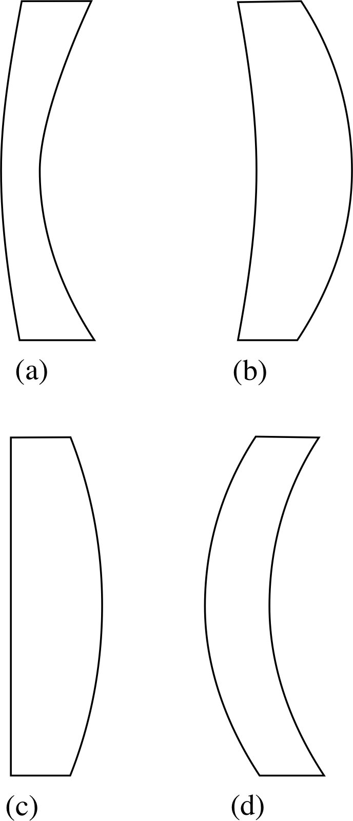
Figure 26 See Answer T4.
Use the lens maker’s equation:
$\dfrac{1}{f} = (\mu-1)\left(\dfrac{1}{r_1}-\dfrac{1}{r_2}\right)$(Eqn 11)
Lens A: 1/f = 0.5[(1/25) − (1/15)] cm−1 = [0.5(3 − 5)/75] cm−1 = (−1/75) cm−1.
So f = −75 cm. The lens is diverging with convex front face and concave back face. (See Figure 26a.)
Lens B: 1/f = 0.5[(1/−10) − (1/−5)] cm−1 = [0.5(−1 + 2)/10] cm−1 = (1/20) cm−1.
So f = 20 cm. The lens is converging with concave front face and convex back face. (See Figure 26b.)
Lens C: 1/f = 0.5[(1/±∞) − (1/−20)] cm−1 = 0.5(0 + 1/20) cm−1 = (1/40) cm−1.
So f = 40 cm. The lens is planoconvex and is converging. Note that the ‘radius of
curvature’ of a plane surface may be taken as ±∞; it makes no difference. (See Figure 26c.)
Lens D: 1/f = 0.5[(1/20) − (1/20)] cm−1 = 0 cm−1.
So f = ∞. The front surface is convex and the rear surface is concave with equal curvature. There is zero net refraction and rays pass through with no change of direction. (See Figure 26d.)
The combination of Equations 10 and 11 (for a given lens) gives the thin lens equation (Equation 12) which relates object distance, image distance and the focal length of the lens.
The thin lens equation$\dfrac{1}{\upsilon} - \dfrac{1}{u} = \dfrac{1}{f}$(12)
This is probably the most important equation in elementary geometrical optics for it shows that if the focal length of a thin lens is known (and it has just been noted how easily that may be measured), then the image position resulting from any object position may readily be calculated.
✦ An object 20 cm to the left of a converging lens produces a real image 10 cm to the right of the lens. What is the focal length of the lens?
✧ u = −20 cm, υ = 10 cm
so1/f = (1/10 cm) − (1/−20 cm) = 3/20 cm.
Sof = 6.66 cm.
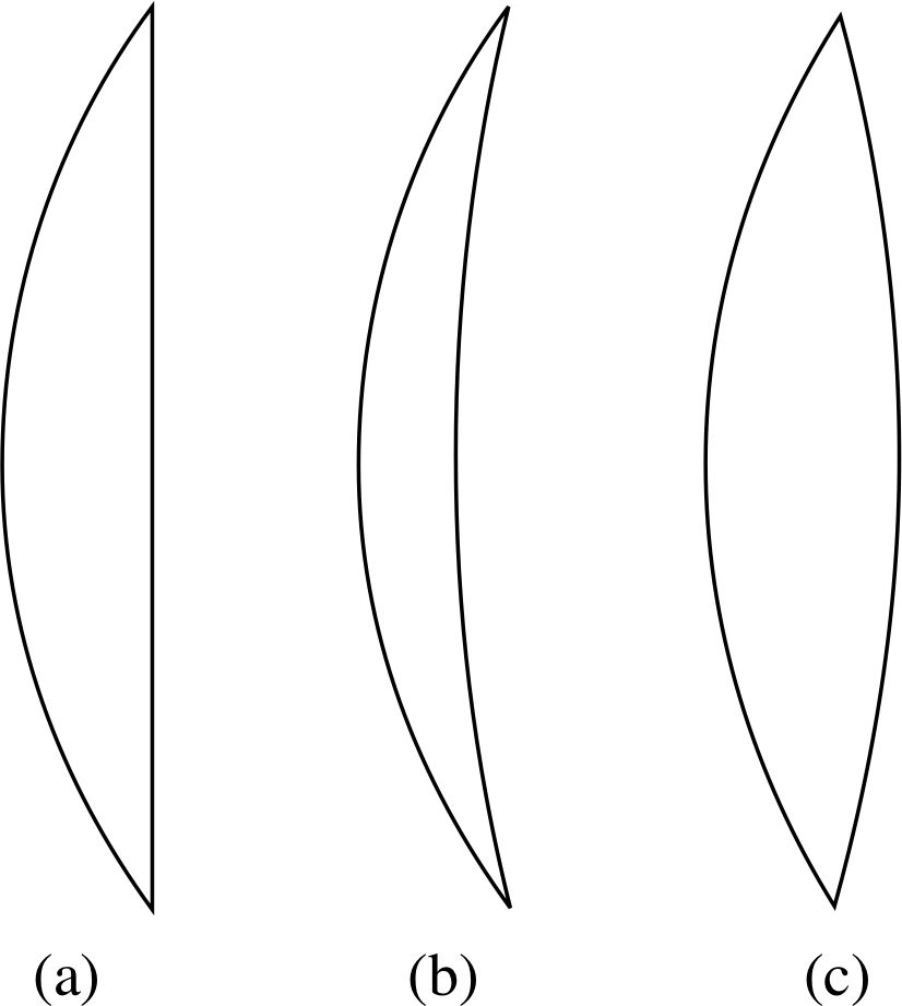
Figure 14 Three types of converging lens:
(a) planoconvex,
(b) convex meniscus and
(c) biconvex.
An object position may be found from which all paraxial rays are refracted by the lens to become parallel to the optical axis, as in Figure 13b. The corresponding image position will be where these parallel rays meet (!) i.e. at infinity, so that 1/υ = 0. The object will then be at the object focus F1, or first focus or first focal point of the lens. The distance of this point from the centre of the lens, obtained by putting 1/υ = 0 in Equation 12, is shown to be equal to −f. Thus the first and second focal points are symmetrically placed on the opposite sides of the lens.
The converging lenses of Figures 12 and 13 are biconvex and may have radii of curvature which are the same for each face or which may differ. It is however not essential for each face to be convex in order for a lens to be converging: the essential requirement is that it should be thicker at the centre than at the edges. This also occurs with two other forms of lens: the plano–convex lens and the convex meniscus lens – see Figure 14.
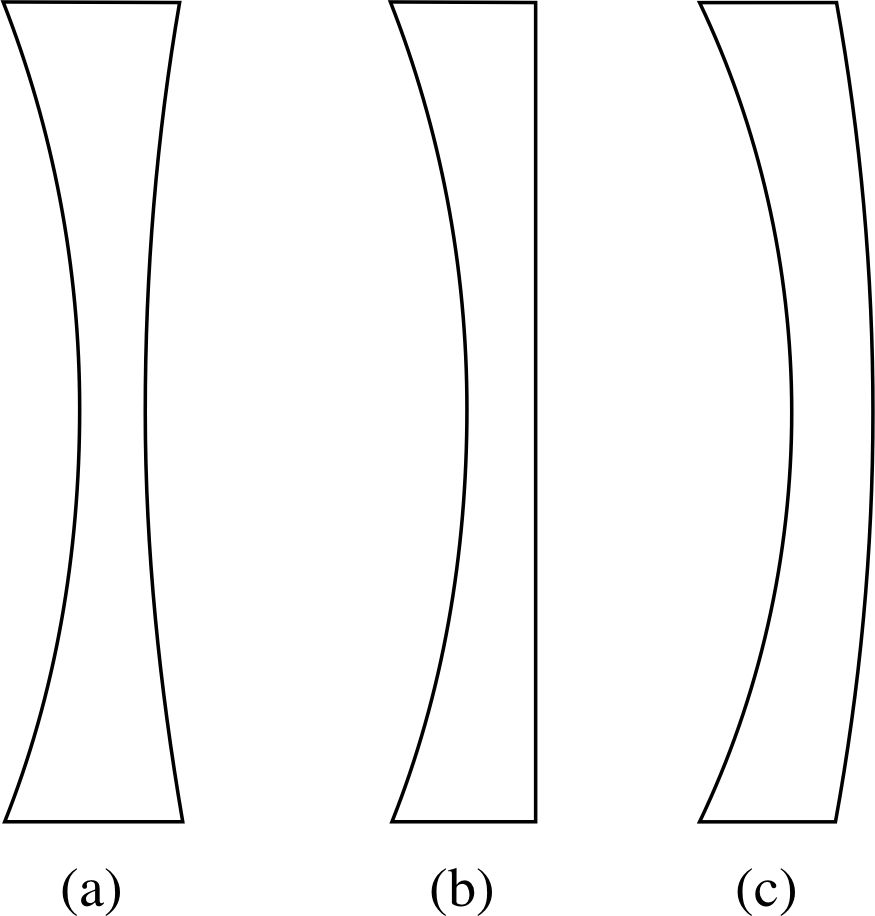
Figure 15 Three types of concave lens:
(a) biconcave,
(b) planoconcave and
(c) concave meniscus.
3.4 Concave lenses
There are three forms of concave lens, namely biconcave_lensbiconcave, plano_concave_lensplano–concave and concave_meniscus_lensconcave meniscus (see Figure 15). Equations 10, 11 and 12, which were derived for convex lenses,
$\dfrac{1}{\upsilon} - \dfrac{1}{u} = (\mu-1)\left(\dfrac{1}{r_1}-\dfrac{1}{r_2}\right)$(Eqn 10)
The lens maker’s equation$\dfrac{1}{f} = (\mu-1)\left(\dfrac{1}{r_1}-\dfrac{1}{r_2}\right)$(Eqn 11)
The thin lens equation$\dfrac{1}{\upsilon} - \dfrac{1}{u} = \dfrac{1}{f}$(Eqn 12)
also apply to concave lenses provided that the correct (negative) sign for focal length is used. Once again the focal length is defined as the distance from the centre of the lens to the second focal point which is generated when incident rays are parallel to the optical axis.
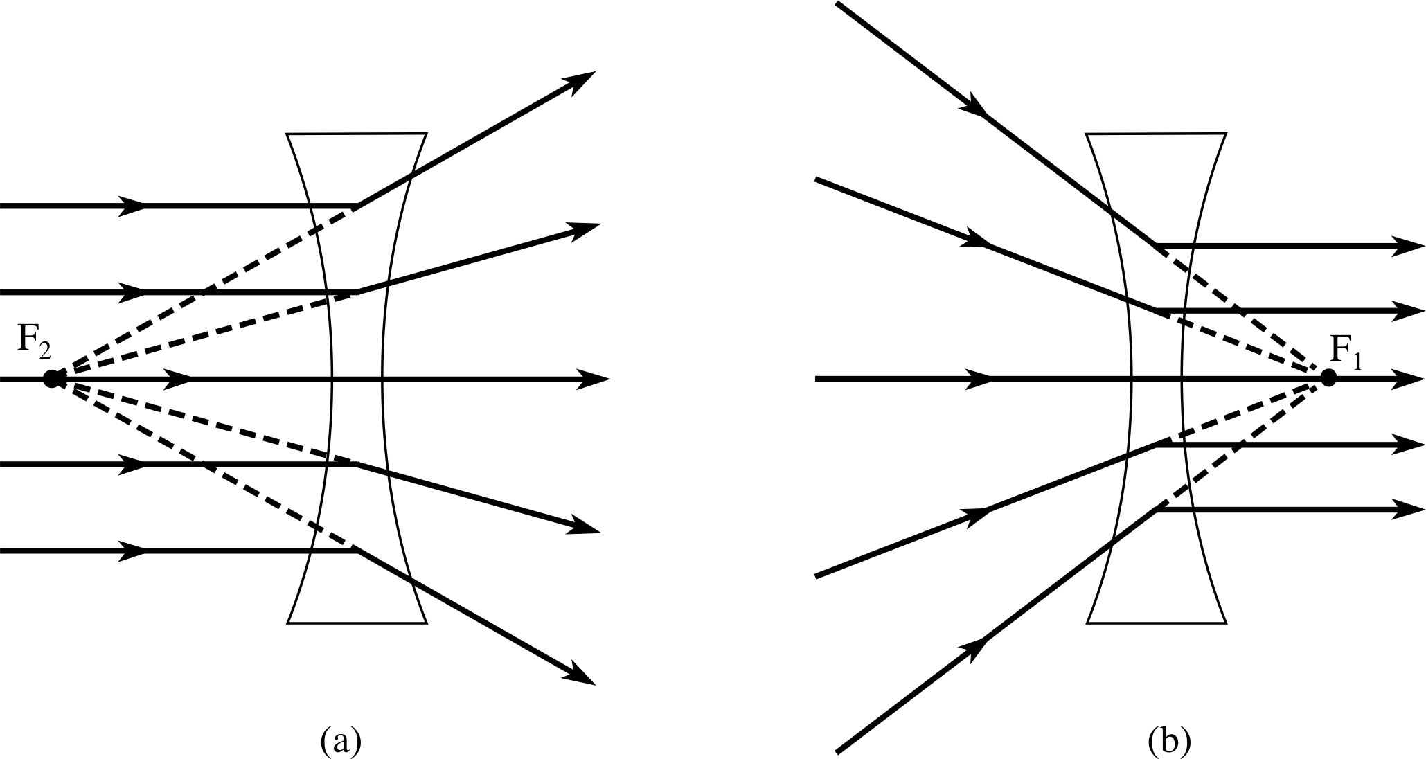
Figure 16 (a) Rays parallel to the optical axis of a concave lens diverge as if from the second focal point F2. (b) Rays converging towards the first focal point of a concave lens are refracted parallel to the optical axis.
However, a concave lens produces a very different ray pattern to that of a convex lens. As shown in Figure 16a, a concave lens causes rays to diverge away from the optical axis and the second focal point F2 is now the point from which the rays appear to diverge.
For a convex lens the first focus is the location at which a point source will generate rays which are refracted by the lens so as to emerge parallel to the optical axis. For a concave lens, the first focus F1 is that point towards which rays must be directed in order that, after refraction at the lens, they follow paths parallel to the optical axis – see Figure 16b. This is another (compare Subsection 3.2) example of a virtual_objectvirtual (point) virtual_objectobject – the rays do not actually meet at F1 – only their projections. i
3.5 Constructing ray diagrams for lenses
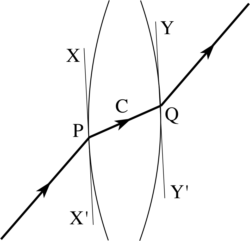
Figure 17 The lateral displacement of a ray through the centre of a thick symmetrical biconvex lens.
We have seen how rays which are parallel to the optical axis pass through, or appear to pass through the first or second focal points of both convex and concave lenses. These rays, together with a third ray through the centre of the lens, are usually called the principal rays and are employed in drawing ray diagrams which enable the relative positions of object, lens and image to be found. If ray diagrams are drawn to scale then they may be used instead of Equation 12 to find the precise position of the image of a particular object. Alternatively, an approximately scaled free–hand sketch provides a quick and easy source of information about the image, as we shall see shortly. Principal rays may be used for both convex and concave lens ray diagrams and, in a modified form, for convex and concave mirrors – as is shown in Subsection 4.4.
The third principal ray is drawn passing through the centre of a lens without deviation or lateral displacement. What actually happens for a biconvex lens, with equal radii of curvature, is shown in Figure 17. In order to show the effect more clearly the thickness of the lens is exaggerated. Tangents XX′ and YY′ have been drawn at the points on the surface of the lens where the ray enters and leaves. Since the ray PQ must pass through the centre of the lens C and the lens is symmetric, the tangents are parallel and the refraction of the ray is the same as if it were passing through a parallel–sided block of glass, i.e. it experiences a small lateral shift but the emergent ray is parallel to the incident ray. For paraxial rays and thin lenses (which may even be asymmetric), this shift is negligible and a ray through the centre of a lens can be represented by a straight line.
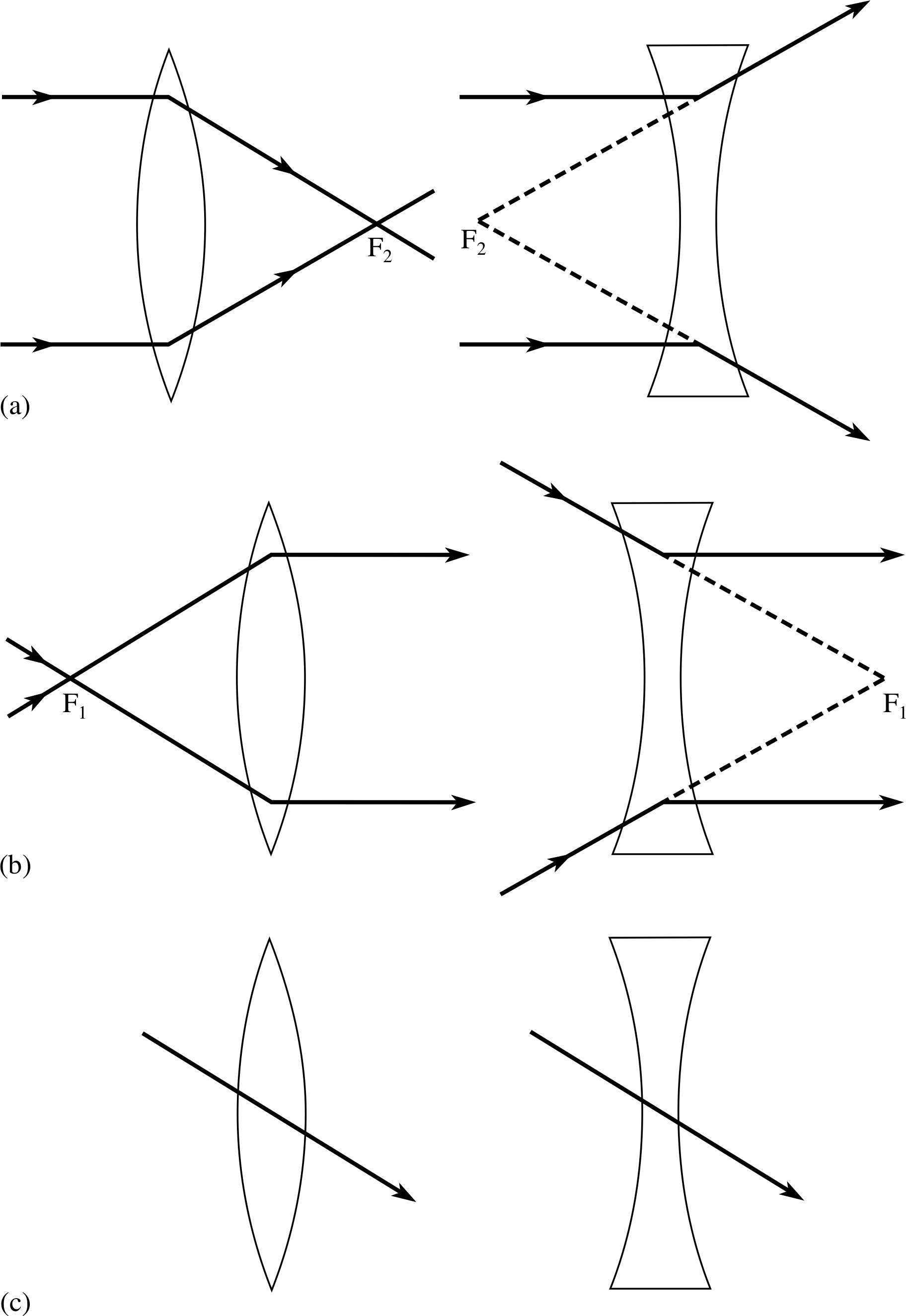
Figure 18 Principal rays used in ray diagrams. Incident rays parallel to the optical axis pass through the second focal point.
Principal rays used in lens ray diagrams:
- 1
-
An incident ray, parallel to the optical axis, emerges from a lens so as to pass directly or by projection through the second focal point.
- 2
-
An incident ray which passes directly or by projection through the first focal point, emerges from the lens in a direction parallel to the optical axis.
- 3
-
A ray passes straight through the centre of a thin lens without deviation or lateral displacement.
Examples of principal rays for converging and diverging lenses are shown in Figure 18.
We are now equipped to find the position of images produced by thin convex and concave lenses for any object position. We have two methods for doing this: we can use either the thin lens equation (Equation 12),
The thin lens equation$\dfrac{1}{\upsilon} - \dfrac{1}{u} = \dfrac{1}{f}$(Eqn 12)
or a ray diagram. If we use the latter, then we will also obtain information about image size and orientation. Practice is required in order to use both methods with confidence, so we start with some examples and follow with some questions.
Example 1: An image formed by a convex lens
Figure 19 Ray diagram for a convex lens with f = 10 cm and u = −15 cm. Note that the zero on the scale bar does not correspond to the origin of Cartesian coordinates which is at C.
The first example, drawn to scale in Figure 19, is a convex lens with a focal length of 10 cm with a real object placed 15 cm from the lens. Being a real object, and therefore the source of light through the system, it is placed to the left of the lens and the object distance is negative, i.e. u = −15 cm. The lens is convex and therefore positive so that f = +10 cm. Substituting these values in the thin lens equation (Equation 12) gives:
$\dfrac1\upsilon = \rm \dfrac{1}{10\,cm}+\dfrac{1}{-15\,cm} = \dfrac{3-2}{30\,cm} = \dfrac{1}{30\,cm}$ so υ = +30 cm
In the ray diagram of Figure 19, the usual practice has been adopted of showing the object as an upright arrow with its base on the optical axis, and it is then described as being erect_imageerect. For clarity and accuracy of drawing, the vertical scale has been much exaggerated – in reality all rays would be paraxial, making angles of not more than about 10° to the optical axis.
Three principal rays are drawn from the point B at the top of the object: BX, a ray parallel to the optical axis is refracted through the second focal point F2; BC, through the centre C of the lens, continues undeviated; BY, an incident ray through the first focal point F1, is refracted to become parallel to the optical axis. All three rays meet at M, which is the image of the point B.
There is no need for further construction to find the position of the remainder of the image as it will be perpendicular to the optical axis, for a perpendicular object.
There are three attributes which may be used to describe an image. These are
- (i)
- its accessibility, i.e. whether it is real or virtual,
- (ii)
- its orientation, i.e. whether it is erect or inverted,
- (iii)
- its magnification, i.e. whether it is enlarged or diminished ( having a dimension perpendicular to the optical axis which is larger or smaller than that of the object).
In Figure 19 we see that IM represents a real image – it could be captured on a screen because the rays we have drawn all come together and pass through M. Secondly, it is upside down so it is inverted, and finally, it is bigger (by a factor of two) than the object, so it is enlarged. We return to this latter point in the next subsection.
As all three principal rays from a point on the object intersect at the corresponding image point, it is only necessary to draw two of them in order to define the image position. It is however instructive to construct all three rays, as this will show how precisely they must be drawn to locate an image position with precision.
Example 2 An image formed by a concave lens
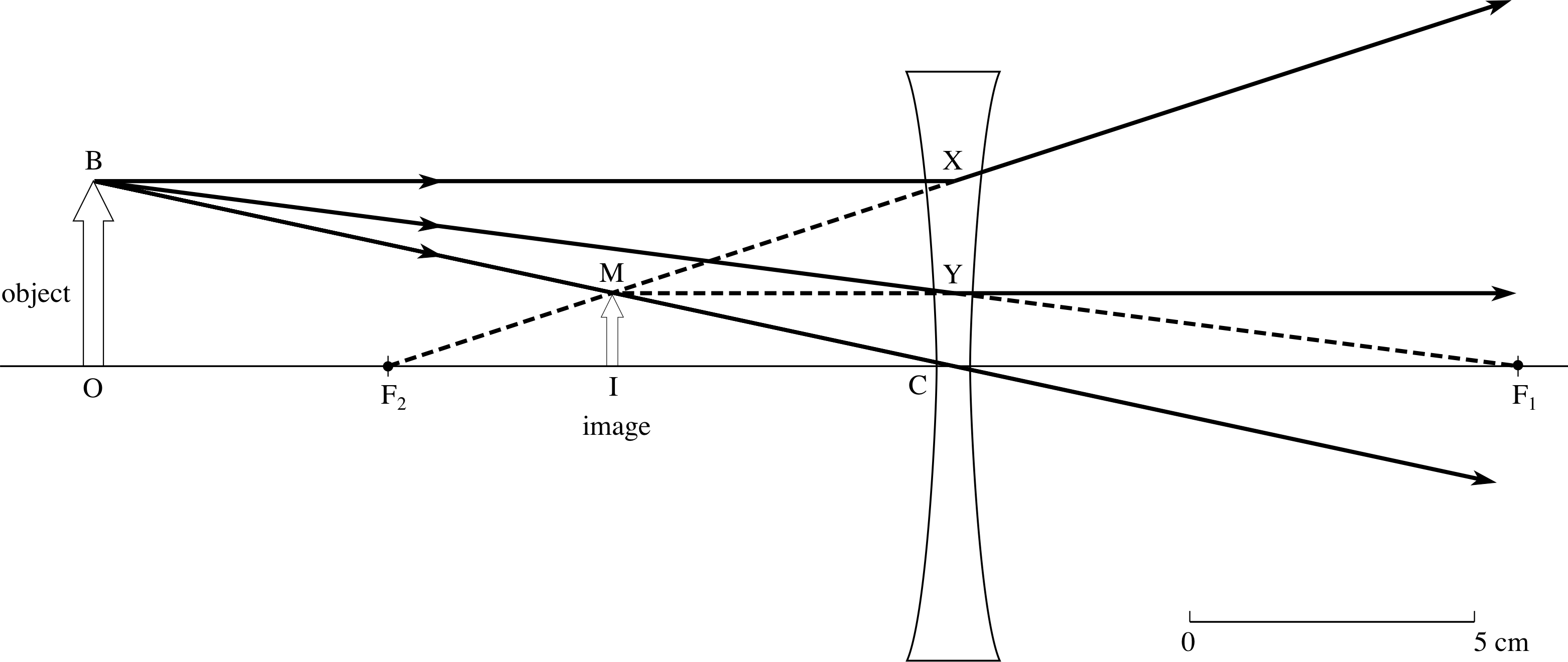
Figure 20 Ray diagram for a concave lens with f = −10 cm and u = −15 cm.
Our second example considers what happens when we replace the convex lens of the first example with a concave lens having the same numerical value of focal length and again with a real object 15 cm from the lens. We insert the values f = −10 cm, u = −15 cm in Equation 12,
The thin lens equation$\dfrac{1}{\upsilon} - \dfrac{1}{u} = \dfrac{1}{f}$(Eqn 12)
which gives:
$\dfrac1\upsilon = \rm \dfrac{1}{-10\,cm}+\dfrac{1}{-15\,cm} = \dfrac{-5}{30\,cm} = \dfrac{1}{30\,cm}$ so υ = −6 cm
All three principal rays are shown in Figure 20. BX is refracted so as to appear to come from F2 and BY is refracted parallel to the optical axis; the back projections of these two rays intersect at M through which BC also passes. The image IM is erect and diminished. It can be seen by looking through the lens but cannot be obtained on a screen and so is virtual.
Example 3 An image of a virtual object formed by a concave lens
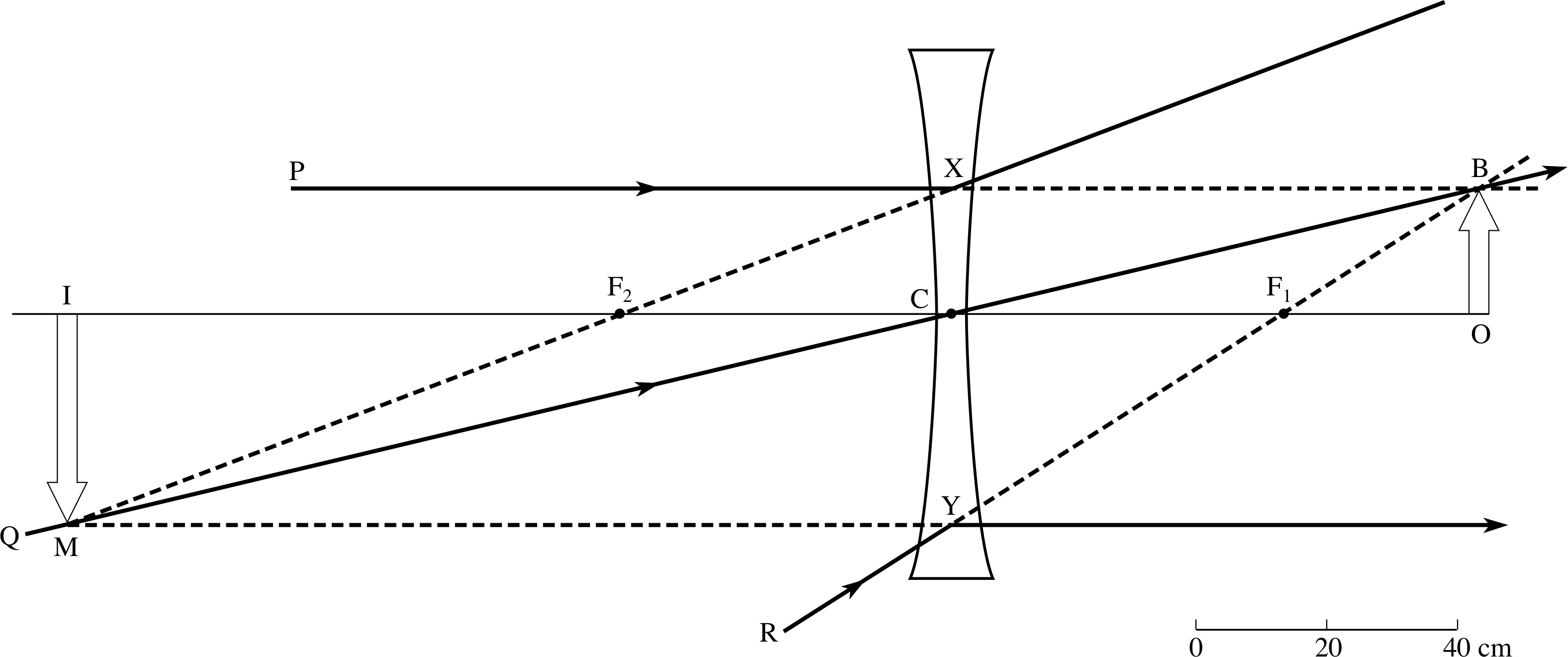
Figure 21 Image formation from a virtual object using a concave lens.
Our third example is shown in Figure 21, in which the rays PX, QC and RY would all have met at the point B and so would have defined the top of a real image OB.
When the concave lens is placed 80 cm in front of OB, the outer rays are made to diverge and appear to come from M. OB therefore serves as a virtual object for the lens, which produces a virtual, inverted and magnified image, IM. The scale of the diagram is such that f = −50 cm, u = +80 cm.
The calculation of the image position is then:
$\dfrac1\upsilon = \rm \dfrac{1}{-50\,cm}+\dfrac{1}{80\,cm} = \dfrac{-8+5}{400\,cm} = \dfrac{-3}{400\,cm}$ so υ = −133 cm
Now see if you can use these methods to answer the following question. i
Question T5
Use both ray diagrams and calculations to find the type and position of the images formed in these systems:
(a) A convex lens of focal length 10 cm with a real object placed 6 cm from the lens, i.e. between F1 and the lens. i
(b) A virtual object located 16 cm from a convex lens of 20 cm focal length.
Figure 27a See Answer T5. A convex lens used as a magnifying glass.
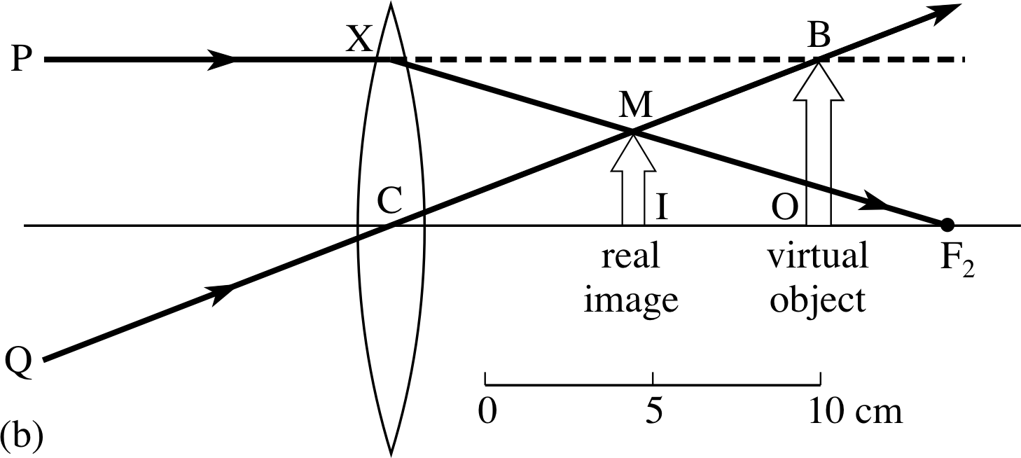
Figure 27b See Answer T5. A convex lens produces a real image of a virtual object.
Answer T5
(a) This is an example of a convex lens used as a magnifying glass. Using Equation 12,
the thin lens equation $\dfrac{1}{\upsilon} - \dfrac{1}{u} = \dfrac{1}{f}$(Eqn 12)
with f = 10 cm and u = −6 cm gives:
1/υ = (1/10 cm) + (1/−6 cm) = (3 − 5)/(30 cm)
1/υ = −2/(30 cm) so that υ = −15 cm.
The ray diagram is shown in Figure 27a.
(b) This is more difficult to visualize, but Equation 12 takes care of the calculation without any difficulties.
As the object is virtual, it must be to the right of the lens, so that u = +16 cm. The focal length f is +20 cm and the equation gives:
1/υ = (1/20 cm) + (1/16 cm) = (4 + 5)/(80 cm)
1/υ = 9/(80 cm), so that υ = 8.9 cm.
To construct the diagram we must choose two rays which would have met at the tip B of the arrow if the lens were not there. Suitable rays are PX and QC in Figure 27b. QC proceeds undeviated to B but PX, being parallel to the optical axis is refracted through F2. The image of the arrow tip is formed at the intersection M of XF2 and CB.
3.6 Transverse magnification by a lens
In the ray diagrams of the previous subsection we saw how the image and object sizes could be very different. Clearly such changes of scale can be of practical importance – the action of many optical instruments such as cinema projectors and microscopes is to create enlarged images; that of the camera is usually to create diminished images.
The transverse dimensions of an image created by a single thin lens are simply related to the transverse object dimensions by the image and object distances.
Figure 19 Ray diagram for a convex lens with f = 10 cm and u = −15 cm. Note that the zero on the scale bar does not correspond to the origin of Cartesian coordinates which is at C.
This may be seen in the simple ray diagram of Figure 19 where the heights of object and image are shown as h and h′, respectively. From the similar triangles OBC and IMC we have h/u = h′/υ. Defining the lens transverse magnification m as the ratio of image height to object height we obtain
lens transverse magnification$m = \dfrac{h'}{h} = \dfrac{\upsilon}{u}$(13)
This expression is applicable to concave and convex lenses, and for both real and imaginary objects and images. If the signs of υ and u are included when calculating m, then it conveys more information than the numerical value of the transverse magnification. Conventionally the object is taken as erect and so if m is positive the image is erect; if m is negative the image is inverted. i
Question T6
Use the scale drawings of Figures 19, 20 and 21 to estimate the transverse magnifications produced by the three lenses in the example calculations (Example 1, Example 2, and Example 3) in Subsection 3.5.
Confirm your results by calculation.
Answer T6
It is a test of the care you have taken with your ray diagrams to see how closely your measured results come to the calculated ones. The precise results obtained from calculation are as follows:
For Figure 19, u = −15 cm, υ = 30 cm, m = 30 cm/(−15 cm) = −2, and the minus indicates an inverted image
For Figure 20, u = −15 cm, υ = −6 cm, m = −6 cm/(−15 cm) = 0.4 and the image is erect.
For Figure 21, u = 80 cm, υ = −133 cm, m = −133 cm/80 cm = −1.66 with an inverted image.
3.7 Optical power
The function of a simple spherical lens is to cause light to converge or diverge, and the shorter the focal length of a lens, the greater its ability to cause this convergence or divergence. Consequently we speak of strong or weak lenses, depending on whether they have short or long focal lengths. The optical power of a lens is defined as the reciprocal of its focal length, and so gives us a quantitative measure which increases with greater converging or diverging ability.
Optical power of a lens$P = \dfrac1f$(14)
If the focal length is measured in metres, then the unit of optical power is the dioptre. Thus a converging lens with a focal length of (+)20 cm has an optical power of +5 dioptres: a diverging lens with a focal length of (−)2.5 m has a power of −0.4 dioptres. The importance of specifying a lens by its optical power will become apparent in the next subsection, when we deal with two lenses in combination.
3.8 Image formation in a two–lens system
Whenever we see an object through some optical system, the final image is formed on the retina of the eye. This means that even for something as simple as a magnifying glass, at least two lenses are involved – the magnifier and your eye lens. To examine the basic concepts involved in analysing multi–lens systems we will consider the simple case of two converging lenses, with the second one placed a distance d along the common optical axis from the first. If the same method of analysis were applied to other lens combinations, identical general expressions would be obtained. The procedure can be extended to systems of more than two lenses.

Figure 22 A two–lens system using converging lenses. Notice that the rays drawn as thick lines are drawn for constructional purposes.
A double lens system is illustrated in Figure 22. The focal length of the first lens is f1 and that of the second lens is f2; the lens separation is d. i As usual, we place an extended object on the left of the first lens at a distance u1 and the light rays go from left to right. The first image is formed at a distance υ1 from the first lens. This image is then taken to be the object for the second lens for which we use a second Cartesian coordinate system with its origin at the centre of the second lens. The object distance for the second lens is u2 = −(d − υ1). Figure 22 shows that the overall linear magnification of this two–lens system is the product of the magnifications produced by each of the two lenses,
Since$\text{overall magnification} = \dfrac{\text{final image size}}{\text{initial object size}} = \dfrac{\rm I_2M_2}{\rm OB} = \dfrac{\rm I_2M_2}{\rm I_1M_1} \times \dfrac{\rm I_1M_1}{\rm OB} = \left(\dfrac{\upsilon_2}{u_2}\right)\left(\dfrac{\upsilon_1}{u_1}\right)$
Applying the thin lens equation (Equation 12),
$\dfrac{1}{\upsilon} - \dfrac{1}{u} = \dfrac{1}{f}$(Eqn 12)
to each lens, we obtain: $\dfrac{1}{\upsilon_1} = \dfrac{1}{f_1} + \dfrac{1}{u_1}\quad\text{and}\quad\dfrac{1}{\upsilon_2} = \dfrac{1}{f_2} + \dfrac{1}{u_2}$
We can eliminate υ1 and u2 by combining these equations, using υ1 = u2 + d to obtain:
$\left(\dfrac{1}{f_1}+\dfrac{1}{u_1}\right)^{-1} - \left(\dfrac{1}{d}\right)^{-1} = \left(\dfrac{1}{\upsilon_2}-\dfrac{1}{f_2}\right)^{-1}$(15)
This is a clumsy equation to use and generally it is better to solve two–lens problems by calculating the position of the first image and then using that as the object position for the second lens calculation, which has been done in the example shown below. The reason that Equation 15 has been quoted here is because, by letting d tend to 0 and rearranging, we obtain a relationship between the initial object and final image distances and the focal lengths of two thin lenses when they are in contact:
$\dfrac{1}{\upsilon_2} - \dfrac{1}{u_1} = \dfrac{1}{f_1} + \dfrac{1}{f_2}$(16)
This equation shows that they behave like a single thin lens which has a focal length f given by:
$\dfrac{1}{f} = \dfrac{1}{f_1} + \dfrac{1}{f_2}$(16)
If we now represent the lenses by their optical powers rather than by their focal lengths, then Equation 17 takes an even simpler form to become:
Presultant = P1 + P2(18)
which states that the resultant optical power of two thin lenses in contact is the sum of their individual powers.
This equation can be extended to include several lenses. i
Notice in Figure 22 that the principal rays (labelled 1 and 2) used in locating the image produced by the first lens are not useful for locating the position of the final image. Two further principal rays (3 and 4) are used for this purpose. These rays can be retraced back through the first lens to the tip of the object, as the figure shows.
The following is an example of a two stage calculation for a two–lens system, similar to that of Figure 22. Treat it as a question if you feel able to do so.
✦ Find the position and magnification of the final image formed by a two–lens system, using the following parameters: f1 = +10 cm, f2 = +7.5 cm, u1 = −15 cm, d = 45 cm.
✧ First apply the thin lens equation (Equation 12) to the first lens:
$\dfrac{1}{\upsilon} - \dfrac{1}{u} = \dfrac{1}{f} = \rm \dfrac{1}{10\,cm}+\dfrac{1}{-15\,cm} = \dfrac{3-2}{30\,cm} = \dfrac{1}{30\,cm}$ so υ1 = 30 cm
The first real image becomes a real object for the second lens:
u2 = −(d − υ1) = −15 cm
Now apply Equation 12 to the second lens:
$\dfrac{1}{\upsilon_2} = \dfrac{1}{f_2}+\dfrac{1}{u_2} = \rm \dfrac{1}{7.5/,cm}+\dfrac{1}{-15\,cm} = \dfrac{2-1}{15\,cm} = \dfrac{1}{15\,cm}$ so υ2 = 15 cm
The second image is real (a sketch will show this) and is located 15 cm to the right of the second lens. The overall magnification of this system is then:
$\dfrac{\upsilon_2}{u_2}\times\dfrac{\upsilon_1}{u_1} = \rm \left[\dfrac{15\,cm}{-15\,cm}\right]\left[\dfrac{30\,cm}{-15\,cm}\right] = 2$
Question T7
A two–lens system is set up as follows: f1 = +10 cm, f2 = +10 cm, u1 = −5 cm, lens separation = 35 cm. Sketch a ray diagram for the system and show that the first image is virtual. Apply the thin lens equation twice to calculate the position of the final image, and then find the overall magnification.
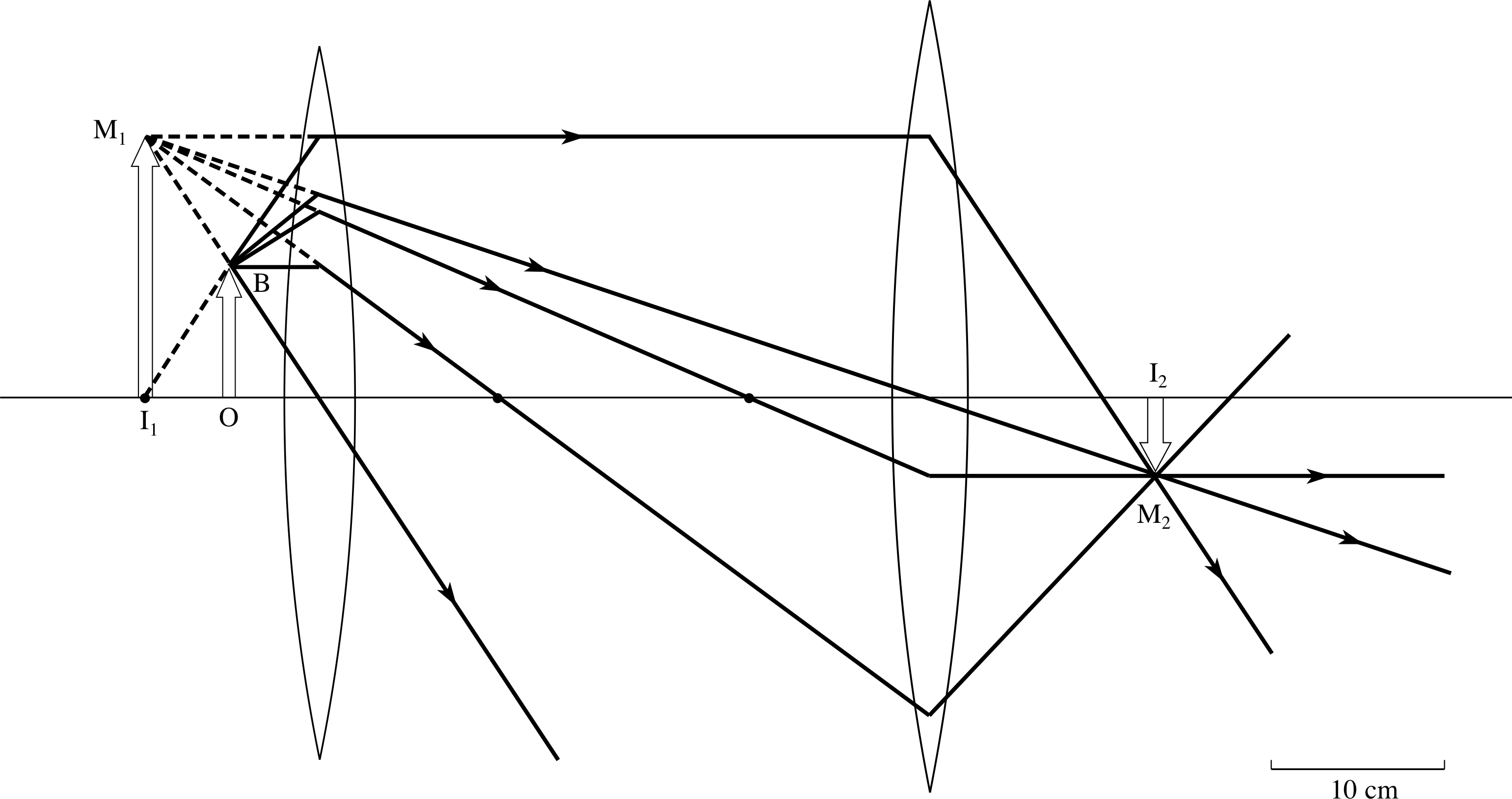
Figure 28 See Answer T7.
Answer T7
Refer to Figure 28. It is necessary to draw two sets of principal rays. The first set is used to locate the first image and the second set to locate the final image produced by the second lens with the first image as the second object.
For the first lens:
1/υ1 = 1/f1 + 1/u1 = (1/10 cm) + (1/−5 cm) = − 1/(10 cm)
soυ1 = −10 cm
The first image is virtual and erect.
The distance of the second object (i.e. the first image) to the second lens is:
u2 = −(d − υ1) = −[35 − (−10)] cm = − 45 cm
1/υ2 = 1/f2 + 1/u2 = (1/10 cm) + (1/−45 cm)
1/υ2 = (9 − 2)/(90 cm) = 7/(90 cm)
soυ2 = 12.9 cm
The final image is real, inverted and to the right of the second lens. The overall magnification is given by the product of the separate magnifications of the two lenses:
m = m1m2 = (υ1/u1)(υ2/u2) = [(−10 cm)/(−5 cm)][12.9 cm/(−45 cm)] = −0.57
The final real image is reduced in size by a factor 0.57 and it is inverted as the minus sign indicates.
4 Reflection at spherical mirrors
The positions of the real or virtual images of extended objects formed by mirrors with surfaces of spherical form (i.e. spherical mirrors) may be studied using methods similar to those developed for thin lenses, keeping to the paraxial (small angle) approximation. However, it should be noted that it is relatively easy to make large mirrors with a parabolic shape (i.e. non-spherical) which make sharp images of point objects on the axis even when large angle rays are included. This is why very large parabolic mirrors are used in optical telescopes where a large light collecting area is desirable. The trigonometry of parabolic mirrors is more complicated than that for spherical mirrors so we will stay with the latter to learn the basic physics of curved mirrors.
The behaviour of light rays at curved mirrors can be summarized as:
- 1
-
A ray incident on a curved mirror surface is reflected as if there were a plane mirror, tangential to the surface, at the point of incidence.
- 2
-
Consequently, incident and reflected rays obey the laws of reflection for plane surfaces, and make equal angles to the normal at the point of incidence. The incident ray, the normal to the surface, and the reflected ray all lie in the same plane.
- 3
-
A normal to a curved surface passes through the centre of curvature for that part of the surface; all normals to a spherical surface pass through the same common centre of curvature.
4.1 A spherical convex mirror
Figure 23 shows a spherical convex mirror. The convex surface bulges out at the centre towards the object, which is conventionally placed to the left of the mirror. As usual, we use the paraxial approximation, which means that all rays considered are either parallel to or make small angles to the optical axis.
This in turn implies that the outward bulge of the mirror is much less than its diameter so that rays at small angles to the optical axis still make small angles to the optical axis after reflection. The radius of curvature of the mirror is r and the centre of curvature is at R.
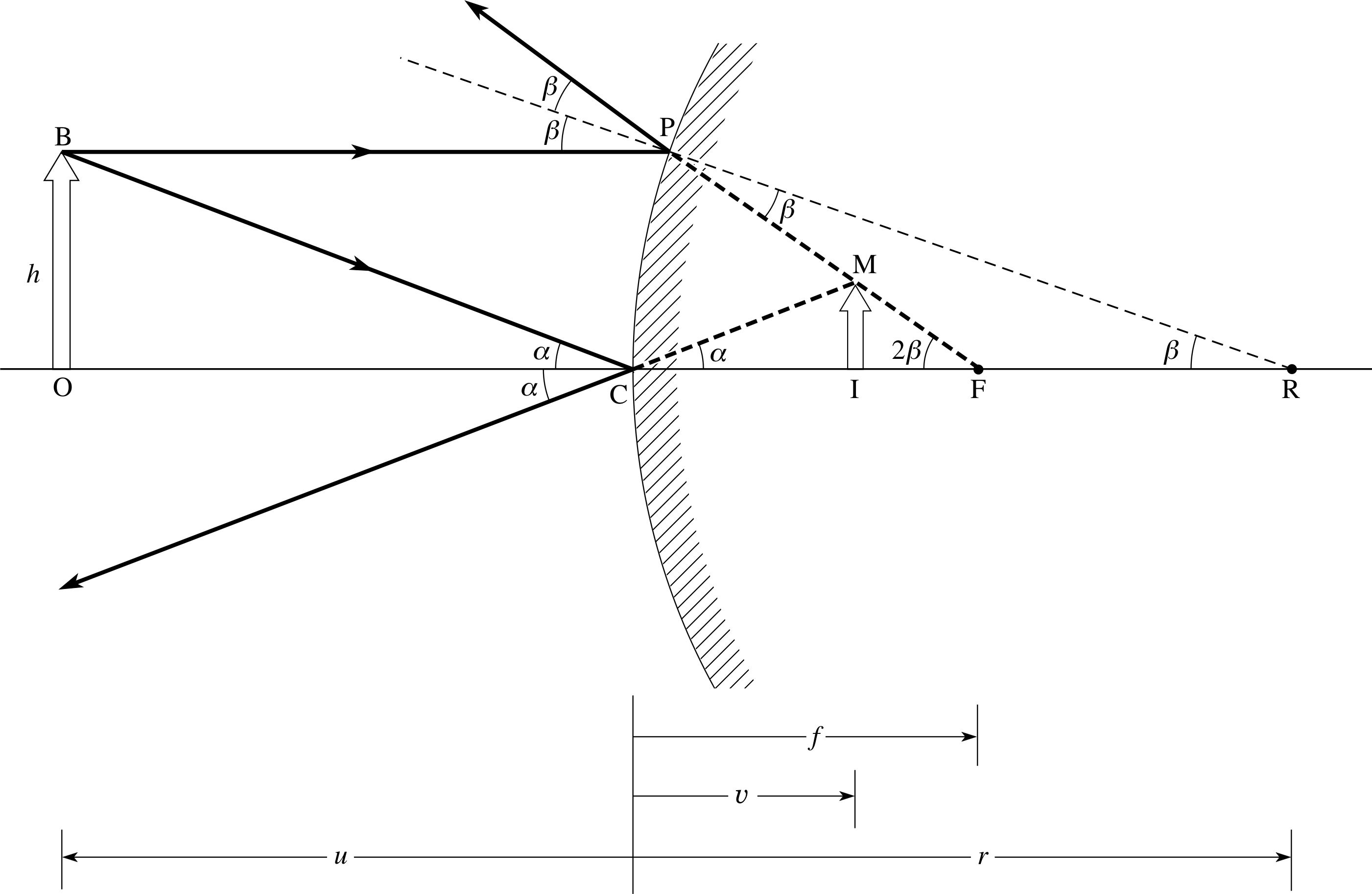
Figure 23 A spherical convex mirror makes a virtual, erect image IM of a real object OB.
The position of an image point is fully determined by the intersection of any two rays from an object point. Consider ray BP which is parallel to the axis from the tip B of the arrow which forms the extended object. This ray strikes the mirror at P where RP is the normal to the surface at the point of incidence. It is reflected away at angle β on the other side of the normal, as though from a point F on the axis. From the triangles PCF and PCR, putting angles equal to their tangents we then have:
2β = tan 2β = h/CF
andβ = tan β = h/CR
where h = CP
Putting CF = f and CR = r, then gives f = r/2.
This is an important result, for it shows that the ray parallel to the axis and reflected at P appears to come from a point halfway between the vertex of the mirror and its centre of curvature. In addition, the expression for f does not involve h, so in the paraxial approximation any ray parallel to the axis is reflected so as to appear to originate at F. We therefore define f as the focal length of the mirror and the point F as the mirror’s focal point. Ray BC, which is directed towards the vertex C of the mirror at an angle α to the axis, is reflected at the same angle below the optical axis, since the axis is normal to the mirror surface at C. Rays BP and BC appear to diverge from the virtual image point at M. Similar ray diagrams and analysis would apply for any object point between B and O and therefore an extended, erect virtual image IM of the extended object OB is formed.
From the trigonometry of triangles OBC and IMC we can obtain the image distance υ in terms of the object distance u, the distance CF = f, and the height of the object OB. Note that in doing so we will, for the moment, treat u, υ and f as positive quantities since we have not yet introduced the appropriate sign convention for mirrors.
We will eventually reintroduce the Cartesian sign convention, but not until it can be properly justified, in Subsection 4.3. For now, note that $\alpha = \dfrac{\rm OB}{u} = \dfrac{\rm IM}{\upsilon}$, so that ${\rm IM} = \dfrac{{\rm OB} \times\upsilon}{u}$.
Also, from above we have $2\beta = \dfrac{\rm CP}{\rm CF}= \dfrac{\rm OB}{f}$ and, from triangle IMF, $2\beta = \dfrac{\rm IM}{f-\upsilon}$
Combining these two expressions for IM, $\dfrac{{\rm OB}\times\upsilon}{u} = \dfrac{{\rm OB}\times( f-\upsilon)}{f}$
which, on dividing by OB × υ, then gives:
$\dfrac{1}{u} - \dfrac{1}{\upsilon} = -\dfrac1f$(19) i
Question T8
Calculate the object position if a virtual image appears 15 cm behind a convex mirror with 20 cm focal length.
Answer T8
Use Equation 19,
$\dfrac 1u-\dfrac{1}{\upsilon} = -\dfrac 1f$(Eqn 19)
with f = 20 cm and υ = 15 cm. Then 1/u = (−1/20 cm) + (1/15 cm) = (−3 + 4)/(60 cm) = 1/(60 cm), and u = 60 cm. Remember, this result made no use of the Cartesian sign convention.
4.2 A spherical concave mirror
A spherical concave mirror is shown in Figure 24 with its reflecting surface curving inwards at the centre away from the extended object OB. We can analyse such a system in much the same way as we did for the convex mirror. The two principal paraxial rays BP and BC are shown originating from the tip of the extended object at B. Ray BP starts parallel to the optical axis, is reflected at P towards the axis and passes through the focal point F. Ray BC strikes the mirror at C, making an angle α to the optical axis, and is then reflected at α below the axis. The point of intersection of the two rays defines M as the tip of the image, so that an extended, real, inverted image IM is formed at distance υ from the mirror.
Figure 24 A spherical concave mirror forming a real inverted image of an extended object.
Referring to Figure 24 we can find the image distance υ = IC in terms of the object distance u = OC, f = FC and h = OB.
Thus in triangles OBC and IMC (treating h, u, υ, f and IM as positive):
$\alpha = \dfrac hu = \dfrac{\rm IM}{\upsilon-f}$
so that${\rm IM} = \dfrac{h\upsilon}{u}$
In triangles PCF and IMF:
$2\beta = \dfrac hf = \dfrac{\rm IM}{\upsilon-f}$
giving${\rm IM} = \dfrac{h(\upsilon-f)}{f}$
Equating expressions for IM:
$\dfrac{h\upsilon}{u} = \dfrac{h(\upsilon-f)}{f}$
Then dividing by hυ gives us:
$\dfrac{1}{\upsilon} + \dfrac{1}{u} = \dfrac1f$(20) i
Again we can use the equations β = h/r and 2β = h/f to show that the length f is half the radius of curvature. For paraxial rays, because f is independent of h, it is defined as the focal length and F as the focal point of the concave mirror.
4.3 The sign convention and mirror calculations
For lenses, it was possible to develop a single formula relating object and image distances for both convex and concave lenses by using a particular sign convention. The same is true for mirrors and we will adopt the same convention as before, which is to use Cartesian coordinates with origin at the mirror’s vertex. Distance of objects, images, focal points or centres of curvature to the right of the vertex are then taken as positive and those to the left as negative.
Equations 19 and 20,
$\dfrac{1}{\upsilon} - \dfrac{1}{u} = \dfrac1f$(Eqn 19)
$\dfrac{1}{\upsilon} + \dfrac{1}{u} = \dfrac1f$(Eqn 20)
may now be written in accordance with this convention.
Thus for the convex mirror of Figure 23, u is negative whereas both υ and f are positive. This modifies Equation 19, so that it becomes:
$\dfrac{1}{\upsilon} + \dfrac{1}{u} = \dfrac1f$(Eqn 21a)
For a concave mirror, with object and image positions as in Figure 24, u, υ and f are all negative so that Equation 20 is unchanged and is identical to Equation 21a.
There are other possible conjugate object and image positions for a concave mirror (e.g. with a virtual object or image) which have not been discussed here. However, analysis of all the possible arrangements will yield equations which, when modified by the Cartesian sign convention, are identical to Equation 21a.
This becomes the spherical mirror equation, the general equation for convex or concave spherical mirrors for paraxial object/image locations.
spherical mirror equation$\dfrac{1}{\upsilon} + \dfrac{1}{u} = \dfrac1f = \dfrac2r$(21b) i
We need to note carefully that this mirror equation is not identical to Equation 12,
the thin lens equation$\dfrac{1}{\upsilon} - \dfrac{1}{u} = \dfrac{1}{f}$(Eqn 12)
because of a difference in signs.
Question T9
Calculate the position of the image in a concave mirror of focal length 20 cm in the following cases: (a) u = −30 cm, (b) u = −15 cm, (c) u = −∞. In each case state if the image is real or virtual.
Answer T9
Use Equation 21a,
$\dfrac{1}{\upsilon}-\dfrac 1u = \dfrac 1f$(Eqn 21a)
with f = −20 cm.
(a) u = −30 cm, so 1/υ = (1/−20 cm) − (1/−30 cm) = −1/(60 cm) and υ = −60 cm
The image is in front of the mirror and therefore is real.
(b) Now we have u = −15 cm and the same focal length so 1/υ = 1/(−20 cm) − 1/(−15 cm) = 1/(60 cm) to give
υ = +60 cm, so that the image is to the right of the mirror and is therefore virtual.
(c) With u = −∞, 1/υ = 1/(−20 cm) − 1/(−∞) = −1/(20 cm) and υ = −20 cm. The image is real and at the focus.
4.4 Constructing ray diagrams for mirrors
As with lenses, there are three principal rays which can be used in the construction of ray diagrams for spherical mirrors, and these are summarized below. Only two of the three are needed to relate object, mirror and image positions in a ray diagram.
Principal rays for mirror ray diagrams:
- 1
-
A ray parallel to the optical axis is reflected through, or appears after reflection, to be coming from, the focal point of the mirror.
- 2
-
A ray which is incident at the vertex of the mirror at a given angle to the optical axis, is reflected at the same angle on the other side of the optical axis.
- 3
-
A ray directed through the centre of curvature of the mirror is perpendicular to the mirror at the point of incidence and is reflected back along itself.
4.5 Transverse magnification by a mirror
The transverse magnification m produced in the paraxial approximation was defined for lens systems as the ratio of image height to object height. With this same definition and referring to the mirror diagrams of Figure 23 or 24 we see that:
$\dfrac{\rm IM}{\rm OB} = \dfrac{\upsilon}{u}$ so that:
mirror transverse magnification
$M = \dfrac{\upsilon}{u}$(22)
If the signs of u and υ are included, then M is negative for erect images and positive for inverted images; note that this is opposite to that for lenses.
4.6 Examples of image formation by spherical mirrors
Two examples will illustrate some practical applications of spherical mirrors. The first is the concave ‘vanity’ mirror, frequently used for putting on make–up or for shaving. This has a typical radius of curvature of about 1 m and the object (i.e. your face) is placed between the focal point and the mirror, as shown in the ray diagram of Figure 25. i
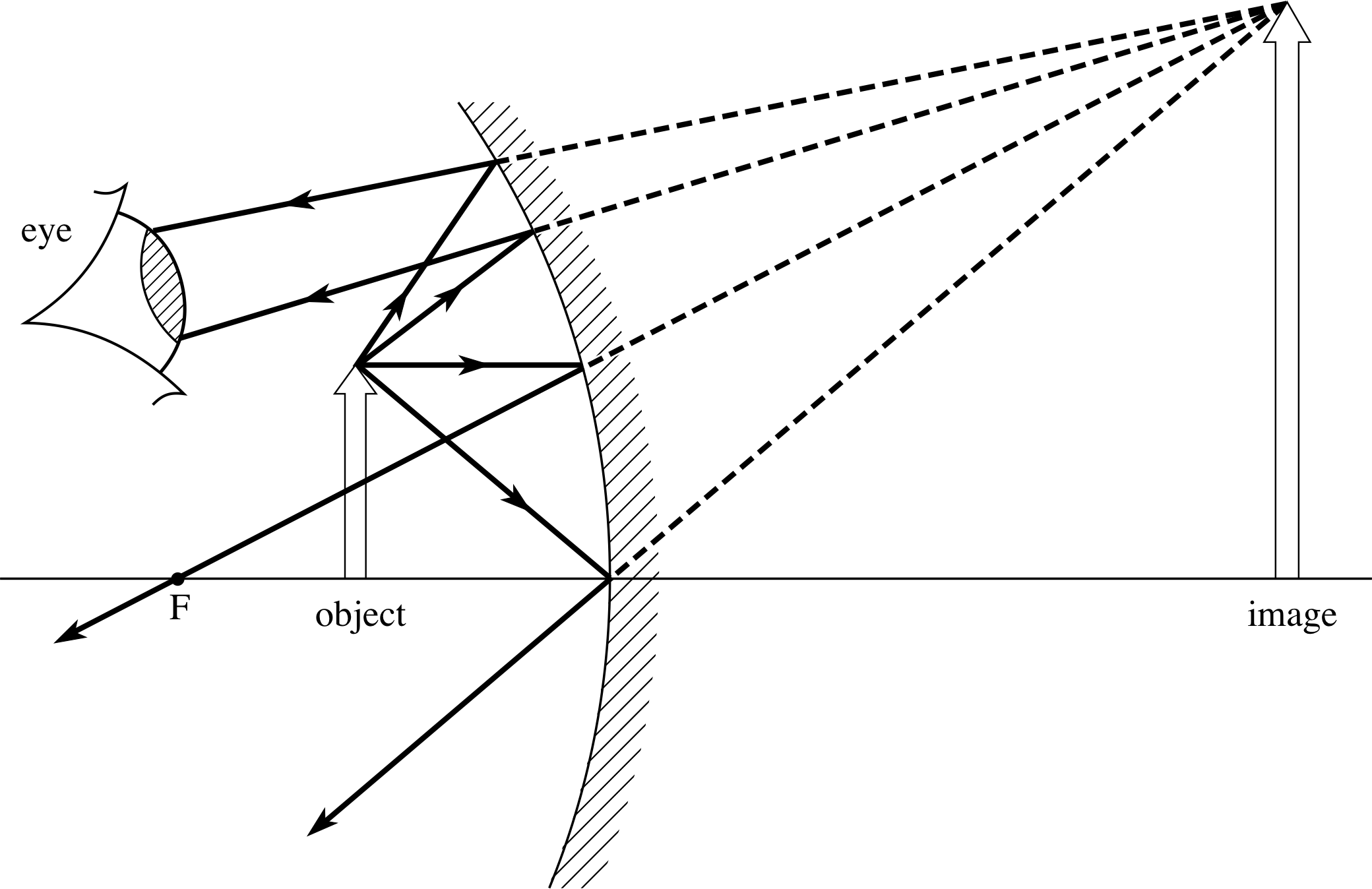
Figure 25 A vanity mirror produces a virtual, erect, magnified image of a nearby extended object (usually your face!)
Inserting the values r = −1 m, u = −30 cm and focal length f = r/2 = −50 cm into the spherical mirror equation,
$\dfrac{1}{\upsilon} + \dfrac{1}{u} = \dfrac1f = \dfrac2r$(Eqn 21b)
we obtain the image distance:
$\dfrac{1}{\upsilon} = \dfrac1f - \dfrac1u = \rm \dfrac{1}{-50\,cm}-\dfrac{1}{-30\,cm}$
$\phantom{\dfrac{1}{\upsilon} }= \rm \dfrac{-3+5}{150\,cm} = \dfrac{2}{150\,cm}$ so υ = 75 cm
From Equation 22,
$M = \dfrac{\upsilon}{u}$(Eqn 22)
the transverse magnification is:
$M = \dfrac{\upsilon}{u} = \rm \dfrac{+75\,cm}{-30\,cm} = -2.5$
The virtual image is located 75 cm behind the mirror, it is erect and magnified by a factor of 2.5. i
Figure 25 also shows how the virtual image can be seen by your eye. Two additional rays from the tip of the object are reflected into the eye and form a real image on the retina. The virtual image in the mirror acts as a real object for the eye lens. In the real world the vanity mirror is often quite large and our strict requirements for paraxial rays are violated. This is not too serious but results in a rather distorted image being produced, particularly at the edges. i
Figure 23 A spherical convex mirror makes a virtual, erect image IM of a real object OB.
Our second example is the familiar convex ‘rear view’ mirror sometimes fitted to cars. Figure 23 shows the detail of the image position construction, the only difference in our example being that the object is much further away so that angle α is smaller and the image much reduced in size and very near to the focus of the mirror.
The mirror has a typical radius of curvature of +2 m and, in this example, we take as the object a car 100 m away. With r = +2 m and u = −100 m, Equation 21b,
$\dfrac{1}{\upsilon} + \dfrac{1}{u} = \dfrac1f = \dfrac2r$(Eqn 21b)
gives the focal length as f = r/2 = +1 m
The image distance υ can then be obtained:
$\dfrac{1}{\upsilon} = \dfrac1f - \dfrac1u = \rm \dfrac{1}{1\,m}-\dfrac{1}{-100\,m} \approx \dfrac{1}{1\,m}$
so υ = 1 m
Equation 22,
$M = \dfrac{\upsilon}{u}$(Eqn 22)
gives the magnification:
$M = \dfrac{\upsilon}{u} = \rm \dfrac{+1\,m}{-100\,m} = -10^{-2}$
Assuming that a car is 2 m in width, the tiny 2 cm wide virtual erect image is located 1 m behind the mirror. You should now think carefully why this is a good idea: we will return to this topic in the Exit test.
5 Closing items
5.1 Module summary
- 1
-
A monochromatic ray of light passing obliquely through a parallel–sided glass block is Figure 1deviated by equal but opposite amounts at the two faces and so the entering and emerging rays are parallel. The deviations of a ray at the faces of a prism are usually both in the same sense so that quite large overall deviations may be produced. If a ray passes symmetrically through a prism, so that its path in the prism makes equal angles with the two prism faces, then the deviation of the ray is a minimum. Relationships between this angle of minimum deviation, the prism angle and its refractive index are given in Equations 4 and 5. The dependence of the deviation on the refractive index together with the variation of refractive index of glass with wavelength, give rise to the dispersion of white light passing through the prism.
- 2
-
Light rays leaving a point source and crossing a spherical boundary between two transparent media are refracted, and either converge towards an image point or appear to diverge from a point, provided that all rays are paraxial. In the paraxial approximation of geometric optics it is assumed that all rays are parallel to, or make small angles with, the optical axis.
- 3
-
The combination of equations describing refraction at two spherical boundaries which are close to each other, leads to a conjugate equation (Equation 10) relating object and image distances to the radii of curvature of the surfaces of a thin lens.
- 4
-
The image distance for an object at infinity, defines the focal length of a lens, and this, together with the adoption of a Cartesian coordinate system, enables the lens maker’s equation to be derived. This equation gives the focal length of a thin lens in terms of the refractive index of the material of the lens and the radii of curvature of its surfaces:
$\dfrac{1}{f} = (\mu-1)\left(\dfrac{1}{r_1}-\dfrac{1}{r_2}\right)$(Eqn 11)
- 5
-
Rays parallel to the optical axis are deviated by a convex lens towards the axis and converge to a real image point. Parallel rays passing through a concave lens are deviated away from the axis and appear to diverge from a virtual image point. These image points are Subsection 3.3focal points for their respective lenses.
- 6
-
Analysis of ray paths leads to the thin lens equation, which relates object and image distances and the focal length of a thin lens, and which is valid for both convex and concave lenses:
$\dfrac{1}{\upsilon} - \dfrac{1}{u} = \dfrac{1}{f}$(Eqn 12)
- 7
-
The lens transverse magnification is given by:
$m = \dfrac{h'}{h} = \dfrac{\upsilon}{u}$(Eqn 13)
and is positive for erect images. A quantitative description of the strength of a lens is its optical power P = 1/f, expressed in dioptres.
- 8
-
As an alternative to calculation, ray diagrams, which are scale drawings using three principal rays, provide a method of finding image positions and system magnifications. Images are described by three attributes: orientation (erect or inverted), magnification (enlarged or diminished), and accessibility (real or virtual).
- 9
-
Systems consisting of two thin lenses on a common optical axis are analysed by regarding the image of the object produced by the first lens, as an object for the second lens.
- 10
-
The paraxial approximation applied to analyse reflection from a convex mirror and a concave mirror produces relationships between object and image distances and focal lengths which are similar, but not identical, to those for lenses. The Cartesian sign convention leads to a paraxial spherical mirror equation
$\dfrac{1}{\upsilon} + \dfrac{1}{u} = \dfrac1f = \dfrac2r$(Eqn 21b)
The focal lengths of concave and convex mirrors are equal to half their radii of curvature.
- 11
-
Ray diagrams, using three principal rays, provide an alternative method of finding image positions and system magnifications for spherical mirrors.
- 12
-
The mirror transverse magnification is given by:
$M = \dfrac{\upsilon}{u}$(Eqn 22)
and is negative for erect images.
5.2 Achievements
Having completed this module, you should be able to do the following:
- A1
-
Define the terms that are emboldened and flagged in the margins of the module.
- A2
-
Describe and explain the behaviour of a light ray passing through a prism and show how this depends on the wavelength of the light. Calculate the angle of minimum deviation for known values of prism angle and refractive index.
- A3
-
Describe: (i) the behaviour of paraxial light rays passing through spherical boundaries and through converging and diverging lenses and (ii) the formation of real and virtual images.
- A4
-
Recall and use the thin lens equation for any object and image position with any kind of thin lens. Determine the position and size of extended images of extended objects using ray diagrams, and determine the magnification of a lens system.
- A5
-
Recall the lens maker’s equation and use it to calculate the focal length of a lens.
- A6
-
Determine the location of the final image in a two–lens system with a common axis by calculation and by ray diagram. Find the optical power of such a system when the lenses are in contact.
- A7
-
Describe the behaviour of paraxial light rays reflected from convex and concave spherical surface mirrors and the formation of images.
- A8
-
Recall and use the spherical mirror equation for any object and image position for convex and concave spherical mirrors. Determine the position and size of extended images of extended objects using ray diagrams, and determine the magnification in any single mirror system.
- A9
-
Describe how convex and concave spherical mirrors are used in some common practical situations.
Study comment You may now wish to take the following Exit test for this module which tests these Achievements. If you prefer to study the module further before taking this test then return to the topModule contents to review some of the topics.
5.3 Exit test
Study comment Having completed this module, you should be able to answer the following questions each of which tests one or more of the Achievements.
Question E1 (A2)
What is the refractive index of a 60° prism for which the angle of minimum deviation is 41°?
Answer E1
This involves substitution of A = 60°, and Dmin = 41° in Equation 4,
$\mu = \dfrac{\sin\theta_1}{\sin\theta_2} = \dfrac{\sin\left[\frac12 (D_{\rm min}+A)\right]}{\sin\left(\frac12 A\right)}$(Eqn 4)
which then gives:
$\mu = \dfrac{\sin\left[\frac12 (60°+41°)\right]}{\sin\left(\frac12 60°\right)} = \dfrac{\sin50.5°}{\sin30°} = 1.54$
(Reread Subsections 2.1 and 2.2 if you had difficulty with this question.)
Question E2 (A2)
A prism is constructed from crown glass which has refractive index 1.520 at λ = 400 nm (violet) and 1.500 at λ = 700 nm (deep red). Light rays with these two colours are incident on the first face of the prism at 25° to the normal. Calculate the difference between the angles of deviation of the two rays as they enter the prism.
Answer E2
The appropriate form of Snell’s law of refraction for the air to glass boundary is given by Equation 2,
sin θ1 = μ2 sin θ2(Eqn 2)
which can be rearranged as θ2 = arcsin[(sin θ1)/μ2]. Then, for violet light, θ2 = arcsin[(sin 25°)/1.52] = 16.14° and for red light, θ2 = arcsin[(sin 25°)/1.50] = 16.36°, so that the difference between these two values of θ2 is a very small angle of 0.2°.
(Reread Subsection 2.1 if you had difficulty with this question.)
Question E3 (A3 and A4)
It is required to make a real inverted image of an extended object using a thin lens. The object is 50 cm from the lens and the image must be double the size of the object. Where is the image and what must be the focal length of the lens?
Answer E3
A converging lens with focal length less than 50 cm is required, otherwise the image will be virtual. There are two unknown quantities, the focal length f and the image distance υ, which can be found using Equations 12 and 13:
The thin lens equation$\dfrac{1}{\upsilon} - \dfrac{1}{u} = \dfrac{1}{f}$(Eqn 12)
lens transverse magnification$m = \dfrac{h'}{h} = \dfrac{\upsilon}{u}$(Eqn 13)
It is given that u = −50 cm and for an inverted image we require m = −2, so that:
1/υ = 1/f + (1/−50 cm) and −2 = υ/(−50 cm), which gives υ = 100 cm.
Hence1/f = (1/50 cm) + (1/100 cm) = 3/(100 cm), and so f = 33.3 cm.
(Reread Subsections 3.2, 3.3 and 3.6 if you had difficulty with this question.)
Question E4 (A4 and A5)
A planoconcave lens, of refractive index 1.50, has the radius of the concave surface equal to 5 cm. Find the focal length of the lens and also its optical power. Show that the magnification of an extended real object is always less than 1.0. What is the magnification when the object is placed 5 cm from the lens?
Answer E4
Use:
the lens maker’s equation$\dfrac{1}{\upsilon} - \dfrac{1}{u} = \dfrac{1}{f}$(Eqn 11)
We are given that r1 = −∞, r2 = +5 cm and μ = 1.50 so that substitution gives f = −10 cm.
The optical power P = 1/f with f in metres, so P = −10 dioptres.
The thin lens equation$\dfrac{1}{\upsilon} - \dfrac{1}{u} = \dfrac{1}{f}$(Eqn 12)
may be rewritten to give the magnification in terms of f and υ:
From 1/υ − 1/u = 1/f we have (u/υ) − 1 = u/f and thus:
u/υ = (u + f )/f
Hence the magnification m = υ/u = f /(u + f ) = 1/[(u/f ) + 1] so that if both u and f are negative, then
m is less than 1.
For the specific case of u = −5 cm:
m = (−10 cm)/[(−5 cm) + (−10 cm)] = 2/3
(Reread Subsections 3.2, 3.3, 3.4, 3.6 and 3.7 if you had difficulty with this question.)
Question E5 (A4)
A screen is placed a fixed distance d from an illuminated object. A thin converging lens is placed between the object and the screen. Show that there are always two positions of the lens at which a sharp image of the object is formed on the screen, provided the focal length is less than d/4. What happens when f is equal to d/4 and when f is greater than d/4?
[Hint: Note that υ − u = d and use the thin lens equation to form a quadratic equation for u.]
Explain why these two lens positions are symmetrically placed about the centre of the system.
Answer E5
Again, we start with:
The thin lens equation$\dfrac{1}{\upsilon} - \dfrac{1}{u} = \dfrac{1}{f}$(Eqn 12)
but add the constraint that the object to image distance is constant, i.e. 1/υ − 1/u = 1/f and (be careful!) υ − u = d. Eliminate υ: 1/(u + d) − 1/u = 1/f, which can be rearranged to give the quadratic equation u2 + ud + fd = 0 which
has two solutions for u:
$u = \left.\left(-d\pm\sqrt{d^2-4fd}\right)\middle/2\right.$
For real solutions d2 ≥ 4fd, i.e. f ≤ d/4.
If we put $k = \left.\left(\sqrt{d^2-4fd}\right)\middle/2\right.$ then the solutions are: u = (−d/2) + k, which makes υ = d + u = (d/2) + k or u = (−d/2) − k, in which case υ = (d/2) − k.
The object and image points are interchangeable. This is because light rays are reversible in a system of lenses. We can reverse the direction of the light ray between a point object and image, the object becomes the image and the image the object!
When f = d/4 there is only one solution to the above quadratic equation: u = −d/2 and this requires the lens to be placed midway between the object and the screen. When f > d/4 there are no real solutions of the quadratic and the lens cannot produce a real image on the screen.
(Reread Subsection 3.3 if you had difficulty with this question.)
Question E6 (A4 and A6)
Two thin lenses, each with focal length +20 cm, are placed 50 cm apart. An object is placed 50 cm from one lens, which makes a real image between the two lenses. Calculate the position of the final image made by the second lens. Is the final image real or virtual?
Answer E6
For the first lens: 1/υ = 1/f + 1/u = (1/20 cm) + (1/−50 cm) = (5 − 2)/(100 cm) = 3/(100 cm), so υ = 33.3 cm
The image from the first lens is treated as the object for the second. For the second lens, the object is at distance u = −(50 − 33.3) cm = −16.7 cm, which is less than the focal length, so the second lens acts as a magnifying glass and produces a virtual image. Substituting we get:
1/υ = 1/f + 1/u = (1/20 cm) + (1/−16.7 cm) = (0.05 − 0.06) cm−1 = −0.01 cm−1 and so υ = −100 cm
confirming that the final image is virtual, inverted and 100 cm to the left of the second lens.
(Reread Subsection 3.8 if you had difficulty with this question.)
Question E7 (A7, A8 and A9)
Older cars possessed wing mirrors, mounted half–way along the bonnet. Explain why it was convenient for such a mirror to be convex, with a radius of curvature of about −2 m, rather than a plane mirror.
Answer E7
The convex mirror produces erect, virtual images of far distant objects about 1 m behind the mirror. The image of a 2 m wide car, 100 m behind you, would be about 2 cm in size. The angular size of an image is defined as the ratio α = (actual size)/(distance from eye).
The driver sits about 2 m from the mirror so α ≈ 0.02/3 ≈ 0.007 radians. In a plane mirror the images have the same angular size as if viewed directly, so α ≈ 2/100 = 0.02 radians. Distant cars appear smaller in the convex mirror. If you can see a 20 m width of the road, at distance 100 m, in a plane rear view mirror then you can see approximately 60 m width in the convex mirror.
(Reread Subsection 4.5 if you had difficulty with this question.)
Question E8 (A7, A8 and A9)
Why is it useful to have a concave mirror to use when shaving or putting on make-up, rather than a plane mirror? Calculate the size of the virtual image of your face when placed 20 cm in front of a concave mirror with radius of curvature −60 cm.
Answer E8
The concave mirror produces magnified, virtual images of an object placed between the mirror surface and its focal point. The virtual image lies behind the mirror. Thus if you put your face close to a vanity mirror you can see your own magnified virtual image. Rays of light diverge from each point on your face, are reflected from the mirror and appear to come from the corresponding virtual image points. Finally the rays converge, after refraction at your eye lens, to form a real image on the retina.
Equation 21b,
spherical mirror equation$\dfrac{1}{\upsilon} + \dfrac{1}{u} = \dfrac1f = \dfrac2r$(Eqn 21b)
gives f = r/2 = −60 cm/2 = −30 cm.
Applying Equation 21b) with u = −20 cm then gives
(1/−20 cm) + 1/υ = (1/−30 cm)
Solving for υ:
1/υ = (1/−30 cm) − (1/−20 cm) = −(2 − 3)/(60 cm) = +1/(60 cm), so υ = 60 cm.
The image is virtual and 60 cm behind the mirror. The magnification is given by M = υ/u = 60 cm/(−20 cm) = −3.
If your face is 25 cm long then the erect virtual image is 75 cm long.
(Reread Subsection 4.5 if you had difficulty with this question.)
Study comment This is the final Exit test question. When you have completed the Exit test go back and try the Subsection 1.2Fast track questions if you have not already done so.
If you have completed both the Fast track questions and the Exit test, then you have finished the module and may leave it here.
Study comment Having seen the Fast track questions you may feel that it would be wiser to follow the normal route through the module and to proceed directly to the following Ready to study? Subsection.
Alternatively, you may still be sufficiently comfortable with the material covered by the module to proceed directly to the Section 5Closing items.