PHYS 5.6: Introducing waves |
PPLATO @ | |||||
PPLATO / FLAP (Flexible Learning Approach To Physics) |
||||||
|
1 Opening items
1.1 Module introduction
The idea of waves is familiar from everyday life, with the most common example being water waves. Most of us have seen ocean waves moving toward a beach, or have generated waves ourselves by dropping stones in a pond. Despite this everyday familiarity, it turns out to be mathematically quite difficult to discuss water waves in detail. In fact, the entire subject of wave motion is rather mathematical. Nonetheless, it is very important that you understand the nature of waves both physically and mathematically, because the concept of a wave is one of the most fundamental and wide–ranging ideas in physics. In this module we examine only the simplest mathematical examples, but they are still quite complicated. It is important at each stage to visualize what the mathematics means, and to keep in mind the underlying physical situation.
We start, in Section 2, by describing certain simple waves mathematically, in a way that is similar to that of simple harmonic motion. In this discussion, we will come to grips with the essential ideas of wave motion. We will concentrate on waves on a string, since these have the virtue of being easy to visualize and relatively easy to describe mathematically. Waves on a string are an example of transverse waves and as such are central to the theme of this module. In the course of studying them you will see how the application of Newton’s laws of motion to waves on a string leads to an equation which describes wave motion in general, and determine the speed of waves on a string.
You will also learn how such investigations involve a mathematical technique known as partial differentiation. (You are not expected to be familiar with this technique, but a limited knowledge of ordinary differentiation is presumed in this module.)
Section 3 is devoted to a fundamental idea in the physics of waves; the principle of superposition. This allows us to regard complicated waves as assemblies of simple waves, and thereby simplifies many problems. It also introduces the important idea of interference between waves.
The superposition principle leads naturally to the discussion of the physical principles behind, and mathematical description of, standing waves. These waves are discussed in Section 4, which also looks at their importance in the context of stringed musical instruments.
Finally, in Section 5, we consider transverse waves in more complicated systems that require more than one dimension for their description. These will include an elastic membrane and waves on water (finally!).
Study comment Having read the introduction you may feel that you are already familiar with the material covered by this module and that you do not need to study it. If so, try the following Fast track questions. If not, proceed directly to the Subsection 1.3Ready to study? Subsection.
1.2 Fast track questions
Study comment Can you answer the following Fast track questions? If you answer the questions successfully you need only glance through the module before looking at the Subsection 6.1Module summary and the Subsection 6.2Achievements. If you are sure that you can meet each of these achievements, try the Subsection 6.3Exit test. If you have difficulty with only one or two of the questions you should follow the guidance given in the answers and read the relevant parts of the module. However, if you have difficulty with more than two of the Exit questions you are strongly advised to study the whole module.
Question F1
A periodic wave is described by the equation
y (x, t) = (3 m) sin[(2 m−1)x − (5 s−1)t]
where y and x are measured in metres and t is measured in seconds. What are the amplitude, wavelength, angular frequency and phase speed of this wave?
Answer F1
The general expression for a sinusoidal wave has the form A sin(kx − ωt), where A is the amplitude, k is the angular wavenumber, and ω is the angular frequency. By comparison with the given equation, the amplitude is 3 m, the angular wavenumber is 2 m−1 and the angular frequency is 5 s−1. The phase speed is given by ω/k, and is thus 2.5 m s−1. Finally, the wavelength is given by 2π/k, and so is equal to π m ≈ 3.14 m.
Question F2
A string has a linear mass density of 0.1 kg m−1 and is under a tension of 500 N. What is the phase speed for transverse sinusoidal waves propagating along this string?
Answer F2
The phase speed is given by:
$\upsilon = \sqrt{\dfrac{F_{\rm T}\os}{\mu}\os} = \rm \sqrt{\dfrac{500\,N}{0.1\,kg\,m^{-1}}} = \sqrt{\dfrac{500\,kg\,m\,s^{-2}}{0.1\,kg\,m^{-1}}} = \sqrt{5000\,m^2\,s^{-2}} \approx 71\,m\,s^{-1}$
Question F3
The string described in Question F2 is held rigidly at the positions x = 0 m and x = 2 m. Describe the motion of the string when transverse standing waves are set up in this segment. What are the allowed linear frequencies and wavelengths of transverse stationary waves on this segment of the string?
Answer F3
The motion of standing waves consists of spatial sine waves along the string for which the length of the string is a multiple of a half-wavelength. Each point along the string undergoes simultaneous simple harmonic oscillations in time. The allowed wavelengths for this string are 4 m, 2 m, 1.33 m, or in general (4 m)/n, where n is any positive integer. The frequencies can be found from the relationship λf = υ.
Here f = 71 m s−1/[(4 m)/n] ≈ 18n Hz.
1.3 Ready to study?
Study comment In order to study this module you will need to be familiar with the following terms from mechanics: acceleration, displacement, energy (kinetic_energykinetic and potential_energypotential), equilibrium, exponential function, force, Newton’s laws of motion, position and work. In addition, you should have a good appreciation of the characteristics of simple harmonic motion. This module is more mathematically demanding than the average FLAP module. You will need to be familiar with the calculus notation dx/dt used to represent the rate of change of x with respect to t, and its interpretation in terms of the gradient of a graph. You should also be able to differentiate simple functions such as sin x and cos x. In the latter part of the module you will be required to use vectors. For the purposes of that section you should know how to express a vector in terms of its components_of_a_vectorcomponents and how to relate those components to the magnitude_of_a_vector_or_vector_quantitymagnitude of the vector. The formal definition of a derivative is used in one subsection and the idea of a scalar product (of two vectors) also makes a brief appearance. Familiarity with both of these items will be helpful but is not essential. If you are uncertain about any of these topics review them in the Glossary, which will indicate where in FLAP they are developed. The following Ready to study questions will allow you to establish whether you need to review some of the topics before embarking on this module.
Question R1
The position of a particle oscillating about a fixed point may be described by the equation x (t) = Acos(ωt + ϕ), where x is measured in metres, and the time t is measured in seconds. If A = 0.1 m, ω = 0.5 s−1 and ϕ = 0.2, i sketch a graph showing how x varies with t for 0 s ≤ t ≤ 15 s and use the graph to explain the physical significance of A, ω and ϕ. What is the period of this motion?
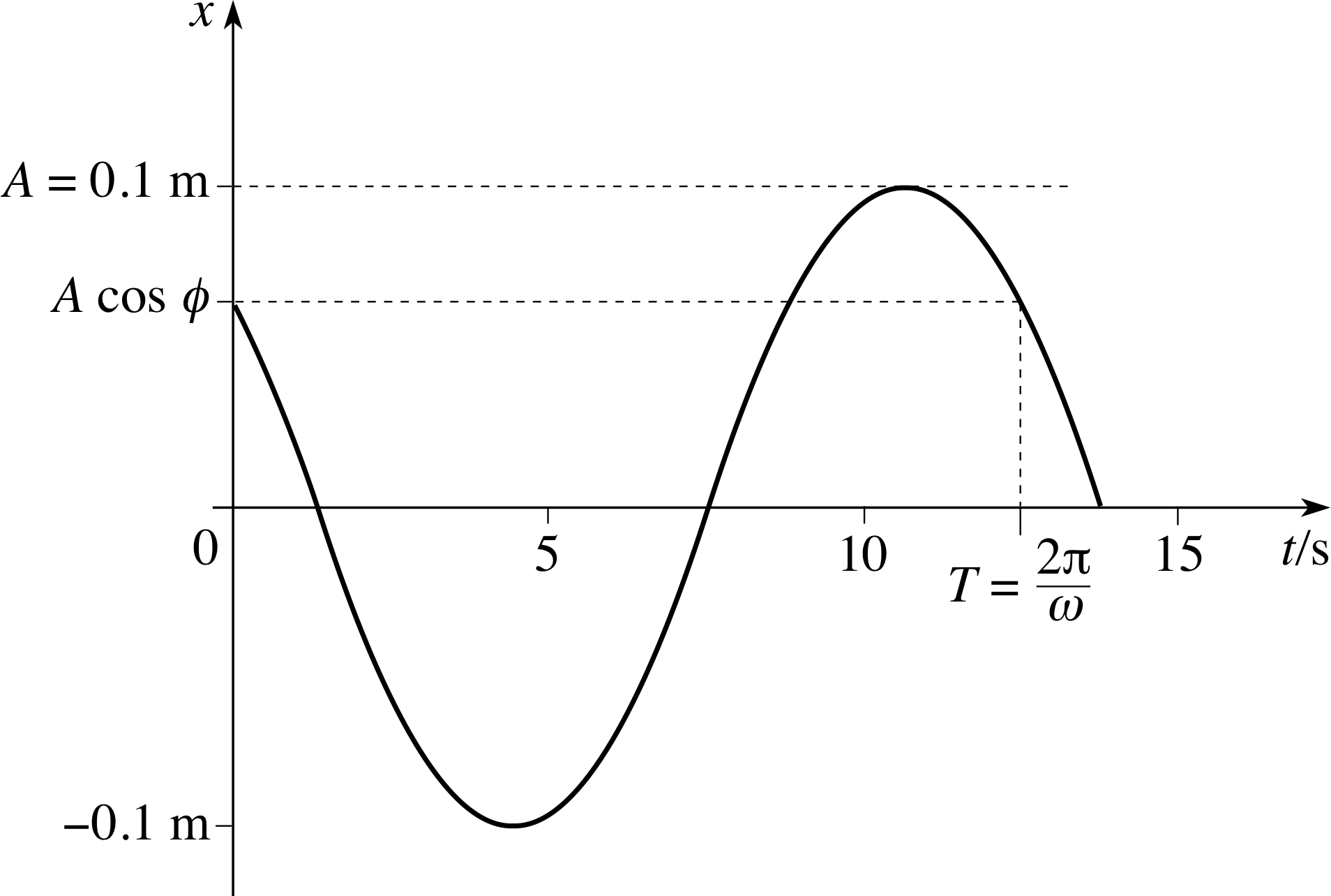
Figure 15 See Answer R1.
Answer R1
See Figure 15 for the sketch of x (t) = A cos(ωt + ϕ).
A is the amplitude: it represents the magnitude of the maximum displacement from the mid–point of the motion. ω is the angular frequency: it is 2π times the frequency of the motion, i.e. 2π times the number of oscillations per second.
(Another way of defining ω is to use f = 1/T, so the angular frequency ω = 2π/T). ϕ is the phase constant or initial phase, it represents the value of the phase (ωt + ϕ) at t = 0, and helps to determine the initial position of the oscillating particle since x (0) = A cos ϕ.
The oscillation described has period T = 2π/ω = 4π s ≈ 12.6 s.
Consult the relevant terms in the Glossary for further information.
Question R2
What is the acceleration of the particle from Question R1 as a function of time? If the particle has a mass of 0.1 kg, what is the force required to produce this motion?
Answer R2
The acceleration is the second derivative of the position with respect to time, which can be calculated as follows:
$\dfrac{dx}{dt} = -A\omega\sin(\omega t+\phi)$
and so$a_x = \dfrac{d^2x}{dt^2} = -A\omega^2\cos(\omega t+\phi)$
i.e.ax = −2.5 × 10⁻² cos(0.5t + 0.2) m s−2
The force required is then
Fx = max = −2.5 ×10⁻² cos(0.5t + 0.2) N
Consult the relevant terms in the Glossary for further information.
Question R3
A straight segment of string lies on a flat surface which we can designate as the (x, y) plane of a coordinate system. Outward forces of magnitude of 10 N are applied parallel to the string at the ends of the segment, which is oriented at an angle of 30° (measured in the anticlockwise sense) to the x–axis. Calculate the x– and y–components_of_a_vectorcomponents of each force and the net force applied to the string segment. What is the magnitude of the tension in the string?
Answer R3
The components_of_a_vectorcomponents of the force can be calculated using Fx = F cos θ, and Fy = F sin θ, where F is the magnitude of the force and θ is the angle the vector makes with the positive x–axis. Let F1 be the vector with in the negative x–component, and F2 that with in the positive x–component. Their respective angles are then 210° and 30° with respect to the positive x–axis. Then we can write:
F1x = (10 N) cos 210° = −8.66 N
F1y = (10 N) sin 210° = −5 N
F2x = (10 N) cos 30° = +8.66 N
F2y = (10 N) sin 30° = +5 N
The net force applied to the string is zero. The magnitude_of_a_vector_or_vector_quantitymagnitude of the tension in the string will be 10 N.
Consult the relevant terms in the Glossary for further information.
2 Travelling transverse waves
2.1 Physical description of travelling waves
We are all familiar with waves. Everyone has a mental image of ocean waves approaching a beach. However, describing such waves physically is not an easy task; even the most basic features of the description are problematic. For example, when a wave approaches a beach, what is it that is actually travelling? It can’t be the water itself, or the entire ocean would gradually accumulate on the beach. Indeed, if you look at small boats or other floating objects you will see that their main response to a passing wave is to move up and down, so it is pretty clear that the movement of the water is essentially vertical – at right angles to the direction in which the wave is travelling. (The water motion is actually slightly more complicated than this, but we will come back to that later.) A similar problem arises when describing the wave that travels along a string or a rope that has been jerked up and down at one end. If one small segment of the string is marked by bright colouring, it can be seen that the marked segment simply moves up and down, it doesn’t travel along with the wave. In the case of ‘mechanical waves’ such as ocean waves and waves on strings, a medium (either the water or the string) is essential to the existence of the wave, but it is clear that the wave does not consist of an overall motion of the medium in the direction of the wave. Moreover, there are waves, such as the electromagnetic waves i associated with light, that can travel through a vacuum and which therefore exist even in the absence of a medium. So, if a wave does not consist of the overall motion of a medium, what is it that does constitute a wave?
When we look at the moving crest of a water wave, we are looking at a region where the surface of the water is raised above its mean (or equilibrium) position. This region of maximum surface displacement certainly moves with the wave, even though the water of which it is composed at any particular moment does not. Similarly, in the case of a wave on a string, it is the location of any point of fixed vertical displacement from the equilibrium position that travels with the wave. Thus, in both these cases the quantity that is ‘waving’ is the vertical displacement of the medium from its equilibrium position. More generally, given a physical quantity with a well defined ‘equilibrium’ value at every point in some region we can say that, as far as that quantity is concerned:
A travelling wave is some sort of disturbance that moves from place to place.
In the case of mechanical waves, and in many other cases, the creation of these wave disturbances requires energy, perhaps to distort a string or to raise a water level, so the movement of such disturbances indicates the transfer of energy from place to place. We can therefore often associate travelling waves with the transfer of energy. In the case of those waves that require a medium, it should be noted that this transfer of energy occurs without a net motion of the medium itself. This kind of energy transfer should be distinguished from that which occurs in streams or rivers (or in water flowing from a tap), in which there is a net motion of the medium.
The displacements that constitute surface waves on water and waves on a string (and the electromagnetic disturbances that account for light waves) all occur at right angles to the direction in which the wave itself is travelling. Any wave with this characteristic is called a transverse wave. Such a wave may be contrasted with a longitudinal wave in which the disturbances are along the direction in which the wave is travelling. (The most familiar example of a longitudinal wave is probably a sound wave which causes molecules to oscillate back and forth around their mean positions.) Longitudinal waves are discussed elsewhere in FLAP; in this module we will almost exclusively be concerned with transverse waves.
2.2 Mathematical description of travelling waves
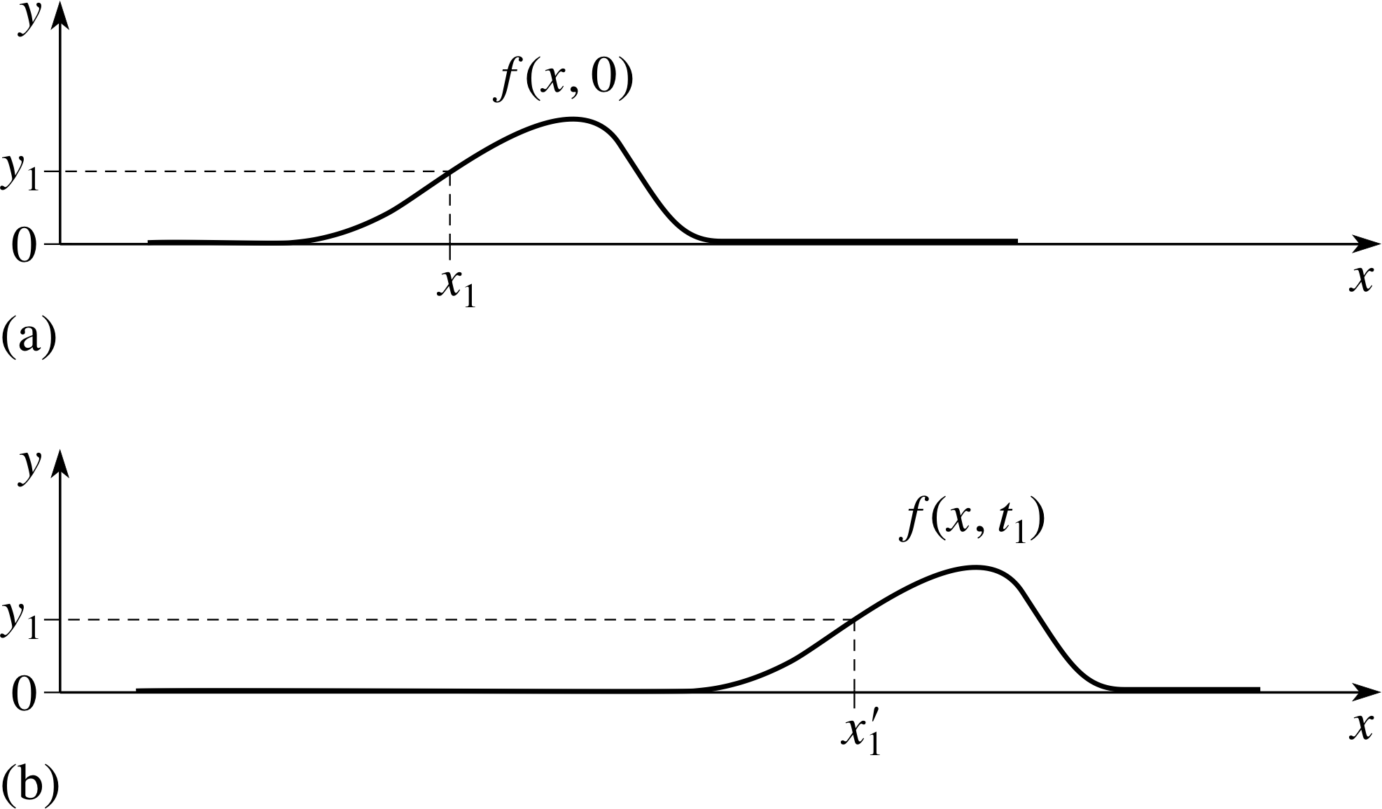
Figure 1 (a) A simple wave pulse on a string at t = 0. (b) The same pulse at a later time t = t1.
We now have a physical picture of transverse travelling waves, but it remains purely qualitative. In order to make it more precise, we need to develop a mathematical description of such waves. As a concrete example, we will look at transverse travelling waves on a horizontal string under tension. To start with we will consider a simple solitary wave (or pulse) in the vertical plane travelling along the string, as shown in Figure 1.
At any particular time, the pulse will have a specific shape or wave profile that can be described mathematically by specifying the vertical displacement y of any part of the string as a function of its horizontal position x.
Note that in introducing the Cartesian coordinates x and y, we have chosen the origin in such a way that x is measured from the left–hand end of the string, and y is measured from the horizontal equilibrium position. With the aid of these coordinates the wave profile at time t = 0 (i.e. Figure 1a) can be represented by y = f (x), where f (x) is the function that relates x to y for this particular pulse. It follows that at a specific point on the x–axis, such as x = x1, we can say that y1 = f (x1) at t = 0.
The wave shown in Figure 1 is moving in the direction of increasing x (hereafter called the +x–direction). This is known as the wave’s direction of propagation and the speed υ with
which it moves in that direction is its speed of propagation. In this case we will assume that υ is constant and that the wave moves without changing its shape. i This combination of constant speed and unchanging shape implies that as time passes the whole pulse moves to the right.
Thus, as Figure 1b indicates, at time t = t1 (x > 0) the part of the pulse with vertical displacement y1 that was initially at x = x1 will be located at some new position x = x1 ′.
✦ Remembering that the speed of propagation is υ, express x1 ′ in terms of x1, υ and t1.
✧ In the time t1, the part of the pulse with vertical displacement y1 will move a distance υt1. So the new position of that part of the wave will be the old position plus the difference υt1. In other words, x1 ′ = x1 + υt1.
We can rearrange this last relationship to give x1 = x1 ′ − υt1. Thus we can write y1 = f (x1) = f (x1 ′ − υt1).
Now there is nothing special about the values x1 and y1 except that they are the coordinates of a point on the wave profile at time t1, so we are justified in saying that at time t1 the entire wave profile (i.e. Figure 1b) can be represented by y = f (x − υt1).
Similarly, there is nothing special about t1 either, so we can say that at any given time t the profile of the entire rightward moving wave is given by
y = f (x − υt) i
A similar line of argument, based on a pulse that has profile y = f (x) at t = 0 but which moves to the left, in the −x–direction, has its profile at any particular time t given by
y = f (x + υt) i
We can therefore say that if a wave with profile y = f (x) at t = 0 moves with constant speed υ and unchanging shape along the +x or −x–direction, then its profile at any time t is given by
y = f (x ± υt)(1)
From a purely mathematical point of view Equation 1 expresses y as a function of two independent variables, x and t. Any mathematical description of a wave must always involve at least two variables since the wave must vary in space as well as in time. (It is this feature that distinguishes a wave from an oscillation in which a displacement or some other disturbance varies with time alone.) As has already been stressed, Equation 1 represents a wave travelling in the ±x–direction with constant speed and unchanging shape. In that case the variables x and t must occur in the combination x ± υt.
However, we can represent more general waves that do not satisfy these assumptions (e.g. waves on a non–uniform string) by an equation of the form y = f (x, t). We can then regard Equation 1as an additional condition that the general function f (x, t) must satisfy if it is to describe waves with constant speed and unchanging shape.
Question T1
Suppose that at t = 0 a wave pulse has the form $f(x) = \dfrac{y_0^3}{x^2 + a^2}$, where y0 and a are both constants. If the pulse moves with unchanging shape with a speed υ in the +x–direction, what will be its mathematical description as a function of time? If υ = 0.5 m s−1, y0 = 0.20 m and a = 0.20 m, sketch the profile of the wave at t = 0 s and t = 4 s.
Figure 15 See Answer T1.
Answer T1
Where x appears in the function, we must insert (x − υt), so the behaviour as a function of time is given by
$y(x,t) = \dfrac{y_0^3}{\left[(x-\upsilon t)^2+a^2\right]}$
At t = 0 this function has a peak value of y = y03/a2 at x = 0. At t = 4 s the entire pulse will have been displaced to the right, the peak will be at x = υt = 2 m, but its shape will be unchanged so its height will be y = y03/a.
The wave profile at t = 0 s and t = 4 s is given in Figure 16.
2.3 Periodic travelling waves
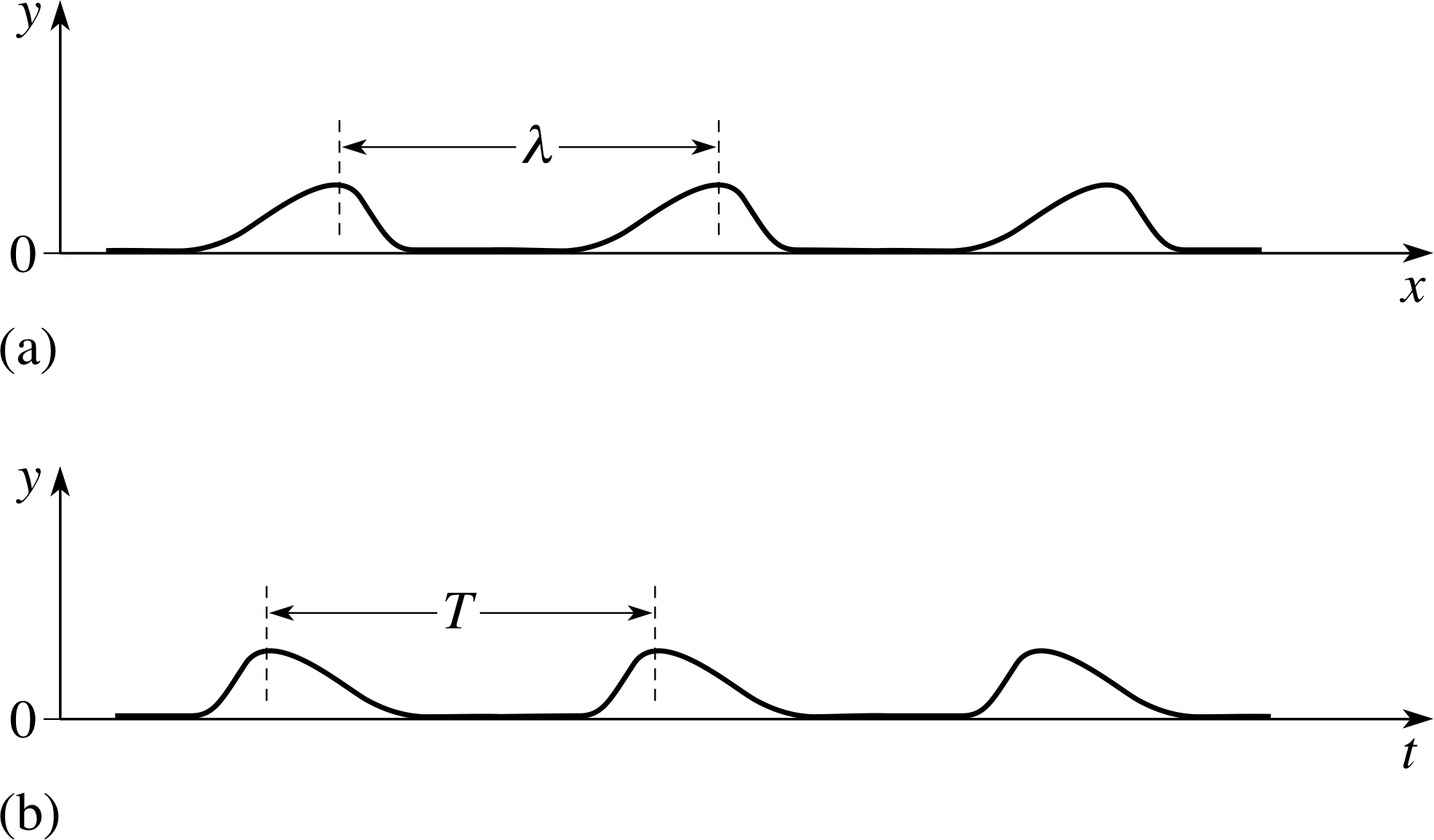
Figure 2 A periodic wave, or wave train. (a) The wave profile at a given time, shows the shape of the wave everywhere on the string at the given time. The wavelength λ is the distance that separates equivalent points on the wave profile. (b) The wave form of the same wave train at a given position, shows the oscillation that the wave causes at all times at the given point. The period T is the time that separates equivalent points on the wave form.
A common feature of waves that we haven’t introduced explicitly yet is the repetition of the wave pattern. Figure 2 shows such a repeating wave, y = f (x, t), made up of a sequence of identical pulses. Since the transverse displacement y varies with time as well as position, the figure shows y as a function of x at a particular time t1 (Figure 2a, the wave profile), and y as a function of t at a particular point x1 (Figure 2b, the wave form.) Repetitive waves of this kind are known as periodic waves or wave trains.
If we consider the wave profile in Figure 2a, we can see that it possesses a spatial periodicity which we can characterize by the wavelength λ.
Mathematically, we can define the wavelength of a periodic wave as the smallest length λ such that:
f (x + λ, t1) = f (x, t1) for all x(2)
This equation expresses the condition that, at a given time, any two points along the wave separated by a distance λ will be completely equivalent. This implies that at a given time, both the transverse displacement and the transverse velocity i will be identical at any two points separated by one wavelength.
Similarly, Figure 2b shows that the wave posses a temporal periodicity which can be characterized by a period T. Mathematically, we can define the period of a periodic wave as the smallest time T such that:
f (x1, t + T) = f (x1, t) for all t(3)
This equation expresses the condition that, at a given point, the wave will cause identical disturbances at any two moments separated by a time T. This implies that at a given point, both the transverse displacement and the transverse velocity will be identical at any two times separated by one period.
We would now like to specialize our description to a particular type of periodic function, namely the sine function. A sinusoidal wave travelling with constant speed υ in the +x–direction (without changing shape) is described by
y = A sin[k (x − υt)](4)
where A and k are constants required to make the expression dimensionally consistent. A is known as the amplitude of the wave; it represents the maximum positive displacement from the equilibrium position and has the same dimensions as the displacement. k is the angular wavenumber; it determines the wavelength of the wave and must have the same dimensions as x−1 to ensure that the argument of the sine function, k (x − υt), is dimensionless. It should be noted that the argument k (x − υt) is called the phase of the wave, and that an even more general kind of sinusoidal wave would be one in which the phase was not necessarily zero at x = 0 and t = 0. Such a sinusoidal wave may be written y = A sin[k (x − υt) + ϕ], where the dimensionless quantity ϕ is called the phase constant. Since the propagation speed υ we have been describing is the speed of a point with fixed phase it may also be referred to as the phase speed.
Question T2
For the wave defined by Equation 4,
y = A sin[k (x − υt)](Eqn 4)
sketch the wave profile at t = 0, and the wave form at x = 0. Use the fact that sin(θ + 2π) = sin θ to show that the wavelength λ and the period T of this wave are related to the angular wavenumber k and the propagation speed υ by the following expressions:
$k = \dfrac{2\pi}{\lambda}\quad\text{and}\quad k\upsilon = \dfrac{2\pi}{T}$
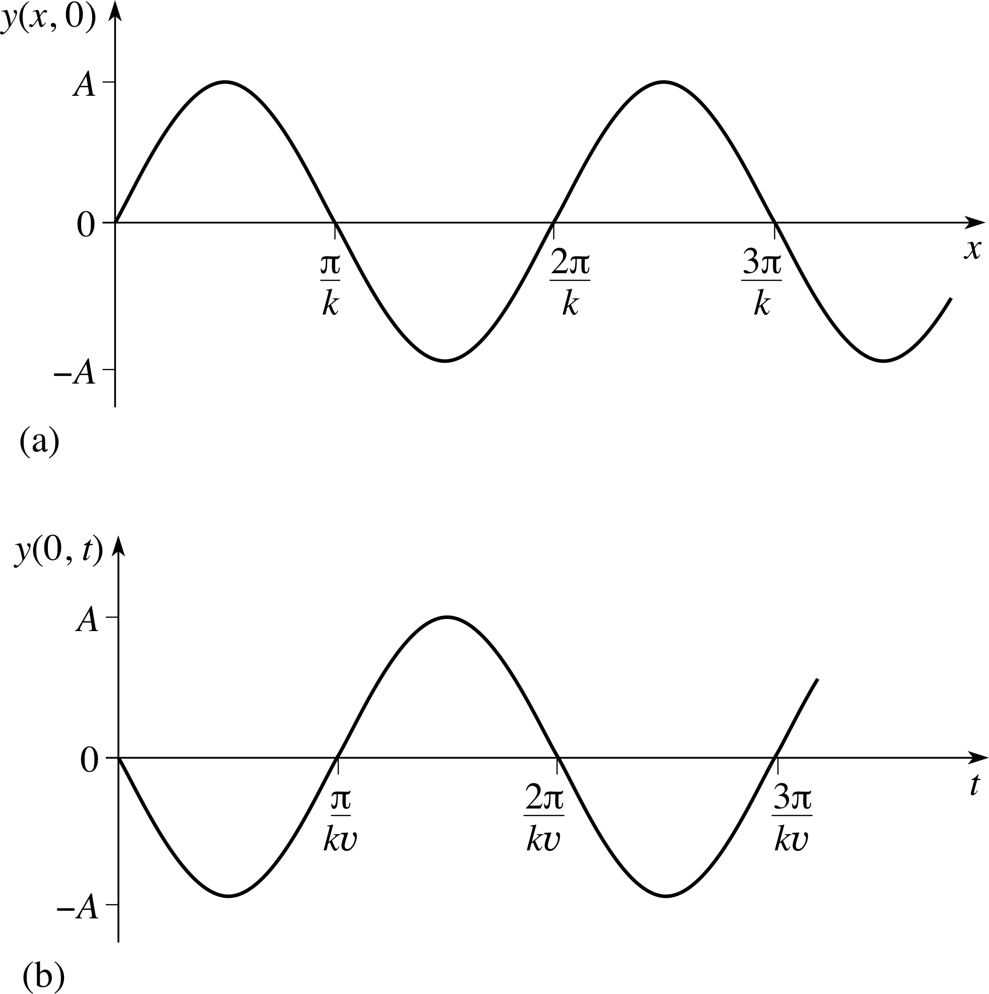
Figure 17 See Answer T2.
Answer T2
The required wave profile is y = A sin(kx), the required wave form is y = A sin(−kυt) = −A sin(kυt). These are shown in Figures 17a and b, respectively. We know that for a general periodic wave f (x + λ, t1) = f (x, t1). Applying this to Equation 4,
y = A sin[k (x − υt)](Eqn 4)
we see that :
A sin[k (x + λ − υt1)] = A sin[k (x − υt1)]
It follows that kλ = 2π, i.e. k = 2π/λ.
Similarly, we know that f (x1, t + T ) = f (x1, t), so for the sinusoidal wave :
A sin[k (x1 − υ (t + T))] = A sin[k (x1 − υt)]
It follows that kυT = 2π, i.e. kυ = 2π/T.
If we examine a sinusoidal wave on a string, and concentrate our attention on any fixed point x, then we find that at that particular point the string is exhibiting simple harmonic motion (you can see this from the wave form that you drew in response to Question T2). The number of oscillations per second occurring at any fixed point is called the frequency and is given by f = 1/T. A related quantity that is also of value in describing these oscillations is the angular frequency ω = 2πf = 2π/T. i
Combining these definitions with the relationships between k, υ, λ and T we can see that:
υ = f λ and $\upsilon = \dfrac{\omega}{k}$
Using υ, T, k, λ, ω and f we may represent the sinusoidal wave in a variety of equivalent ways:
y = A sin[k (x − υt)](Eqn 4)
y = A sin(kx − ωt)(5)
y = A sin[2π (σx − ft)](6)
$y = A\sin\left[2\pi\left(\dfrac x\lambda - ft\right)\right]$(7)
$y = A\sin\left[2\pi\left(\dfrac x\lambda - \dfrac tT\right)\right]$(8) i
If you examine these equations you will see that Equation 6 contains a constant σ that we have not yet defined. Comparing Equations 6 and 7 we see that σ = 1/λ, so it can be thought of as the number of wavelengths per metre. σ is properly called the wavenumber, but unfortunately that term is also widely used to refer to the angular wavenumber k, so make sure you know which is being referred to in any particular situation.
Each of the different descriptions of the sinusoidal wave has its uses, but Equation 5 is probably the most useful to remember as you will generally find that you can work out the other forms if you need them, especially if you also remember the following general relations"
ω = 2π/T and f = 1/T
k = 2π/λ and σ = 1/λ
υ = λf
υ = ω/k(9)
| Variable | Space (x) | Time (t) |
|---|---|---|
| periodicity | λ | T |
| number of linear cycles per unit variable | σ | f |
| number of angular cycles per unit variable | k | ω |
It is worth noting that these relations are generally true for any periodic wave form, not just for sinusoidal waves.
Table 1 summarizes the correspondence between the parameters describing the spatial dependence and those describing the temporal dependence. The space and time parameters are connected through the phase speed.
2.4 Visualizing sinusoidal travelling waves
We now have several equivalent mathematical descriptions of sinusoidal travelling waves. However, in order to understand any of them fully we need to examine them from several different points of view, since they relate the displacement y to two variables x and t. This subsection is intended to help you to visualize these waves.
Imagine a dark room with a horizontal luminescent string stretched across it, from the south wall to the north wall. Now imagine that sinusoidal waves are made to travel along this string, from south to north, and that you are able to see parts of these waves by looking through some rather odd windows in the east and west walls of the room.
✦ The first window lets you see the entire string, but only for a moment – as a kind of snapshot (imagine it has a shutter which opens and closes very quickly). What would you see?
✧ The view shows the wave profile at the moment of observation. You would simply see a luminescent sine wave stretched across the room with successive peaks separated by a distance equal to the wavelength λ.
To understand this mathematically, suppose that the north–south direction is the direction of the x–axis of a coordinate system, and that the y–axis points vertically upwards. If t1 represents the time of observation, then
y = A sin(kx − ωt)(Eqn 5)
takes the form y = A sin(kx − ωt1) which is a sine function in the x–coordinate, with amplitude A and angular wavenumber k = 2π/λ. The constant −ωt1 determines the displacement y at x = 0.
✦ The second window is vertical and very narrow, but it remains open all the time. What would you see?
✧ This view shows just one small part of the luminescent string as it moves up and down executing simple harmonic oscillations with frequency f.
In this case, you are observing at a fixed value of x, so in terms of Equation 5, y = A sin(kx1 − ωt) = A sin(ωt + π − kx1), which describes a sinusoidal motion in time with amplitude A and angular frequency ω. The constant (π − kx1) determines the displacement y at t = 0.
Question T3
Using an appropriate trigonometric identity show that the two sine functions equated above are indeed identical.
Answer T3
Using the identity that sin(θ) = − sin(−θ) and that sin(A − B) = sin A cos B − cos A sin B, we can write:
sin(ωt + π − kx1) = −sin(kx1 − ωt − π)
sin(ωt + π − kx1) = −[sin(kx1 − ωt) cos(−π) − cos(kx1 − ωt) sin(−π)]
sin(ωt + π − kx1) = −[sin(kx1 − ωt)(−1) − cos(kx1 − ωt)(0)] = sin(kx1 − ωt)
✦ The third window is horizontal and very narrow. It allows you to see the entire length of the room at all times, but only at a level slightly above the equilibrium level of the string. What would you see?
✧ This view shows all those parts of the string that simultaneously have the same (positive) value of y. You would see a succession of luminescent segments moving across your field of view, travelling from south to north with the wave’s phase speed υ. i
Each of these three different windows corresponds to holding one of the three variables t, x or y constant, and provides a different view of a travelling wave. Each explicitly shows us one of the characteristic parameters of the wave: frequency, wavelength or phase speed.
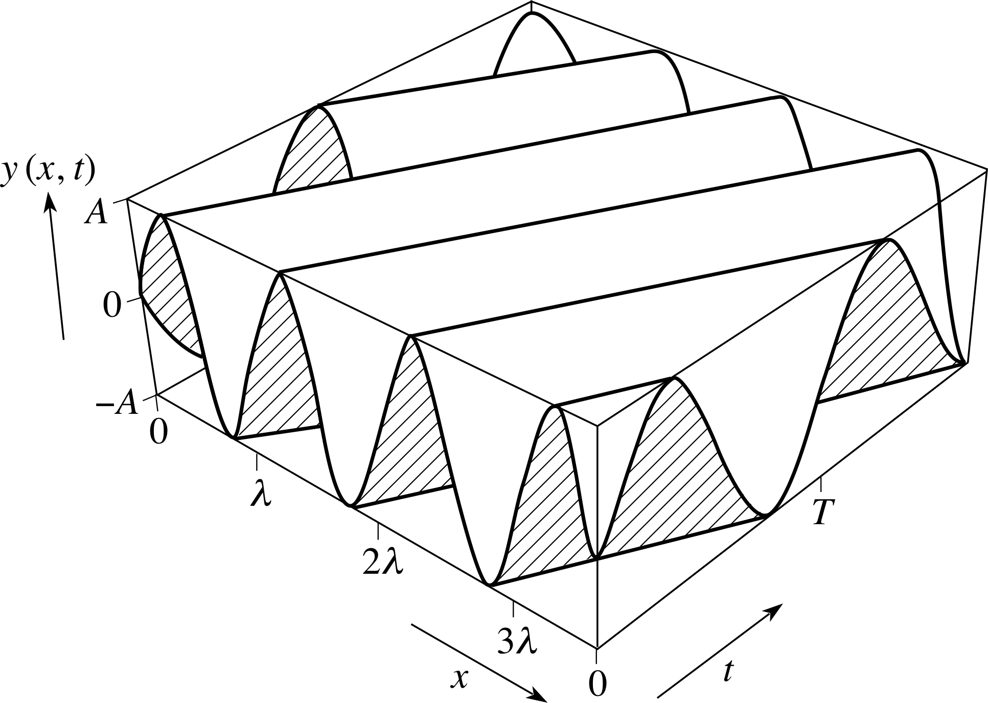
Figure 3 A three–dimensional graph of the function y = A sin(kx − ωt). In this case ω/k = 0.7 m s−1.
An entirely different way of visualizing a function of two variables such as y = A sin(kx − ωt) is in terms of a three–dimensional graph in which the x– and t–axes are located in a horizontal plane and the value of y corresponding to any particular pair of values (x, t) is plotted vertically.
Such a graph is shown in Figure 3. The wave profile at any time is represented by a cross section of this graph taken parallel to the (x, y) plane, at the appropriate value of t. Similarly, the wave form at any particular point is represented by a section taken parallel to the (t, y) plane at the appropriate value of x. Three–dimensional graphs can provide great insight into functions of two variables, but they are difficult to draw and may be even more difficult to interpret.
2.5 The force law for a wave on a string
Study comment This subsection involves some mathematical ideas that may be new to you and which you may find daunting. If so, don’t be put off. If you find it difficult to follow the arguments concentrate on the physical situation that the mathematics is describing. Once you have mastered that, the mathematical formalism should be easier to understand.
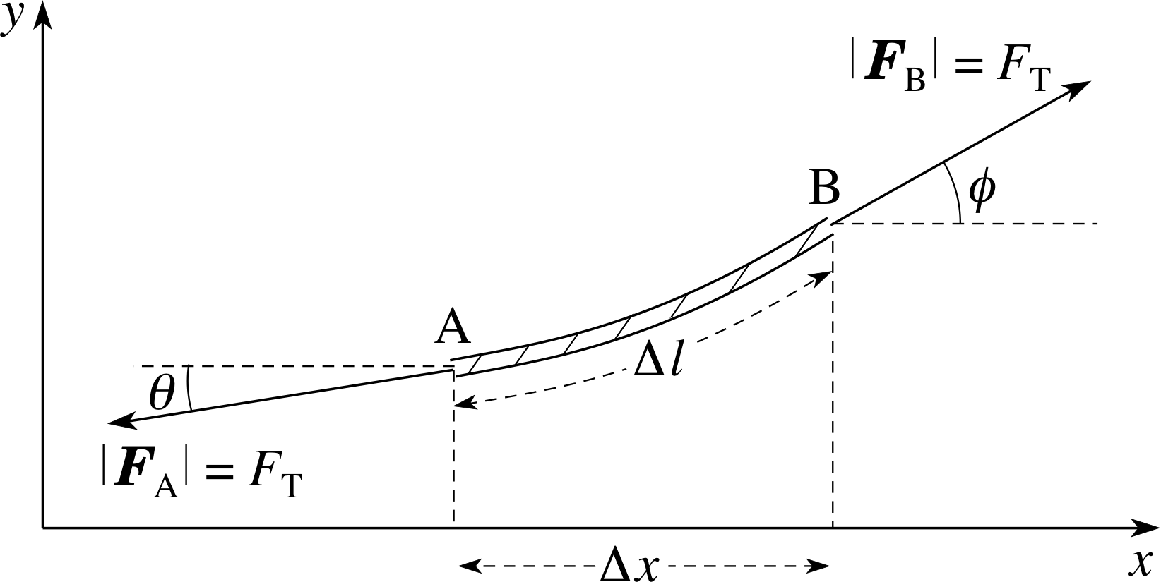
Figure 4 A small segment of string and the forces that act on it due to the tension in the string. Tangents to the string, drawn at the end points A and B of the segment, make angles θ and ϕ with the positive x–axis. The angles in the figure are positive and large enough to be clearly seen, but in principle they might be negative and we shall assume that whatever their sign they are actually very small.
We now have a way of describing the motion of a wave on a string, in other words we have a kinematic description of the wave, but we also would like to be able to understand the causes of the motion, that is to describe the motion dynamically – in terms of the forces that cause it. For a wave on a string this should be possible since we can determine the forces that act on any small segment of the string and then use newtons_laws_of_motionNewton’s laws to work out how the segment will move in response to those forces. By considering what happens when we consider a smaller and smaller segment we should ultimately be able to predict the motion of any point on the string, and hence the behaviour of the wave itself.
Figure 4 shows the sort of small segment of string we wish to consider. The segment will generally be curved, with its ends A and B, respectively, making angles θ and ϕ with the horizontal. i The length of the segment is ∆l and the projection of this length onto the x–axis is ∆x. In order to make the analysis of the motion of this segment as simple as possible, we will make a number of simplifying assumptions: i
- 1
-
We will assume that the tension in the string has the same magnitude at all points. (This can only be an approximation: the passage of the wave will stretch the string slightly, which will increase the tension. However, if the wave is of small amplitude, this will be a small effect which we can ignore.)
- 2
-
We will also assume that the angles ϕ and θ that the string makes with the horizontal are small. This will allow us to make various approximations, including cos θ = 1, cos ϕ = 1 and ∆l = ∆x.
- 3
-
We will ignore the weight of the segment, so the only forces that act upon it are the tension forces on its ends due to the neighbouring parts of the string.
Referring to Figure 4, and remembering that the angles have been exaggerated, you can see that tension forces on the ends of the segment are of equal magnitude, FT, but they act in different directions. At end A the components of the tension force are:
Fx(A) = −FT cos θ and Fy(A) = −FT sin θ
At end B, the corresponding components are:
Fx(B) = FT cos ϕ and Fy(B) = FT sin ϕ
Since the angles are small and cos θ = cos ϕ = 1 it follows that the total horizontal force on the segment is
Fx(A) + Fx(B) = 0
It follows from Newton’s second law of motion, F = ma, that the segment will have no tendency to accelerate in the x–direction.
On the other hand, the y–component of the total force on the segment is
Fy(A) + Fy(B) = −FT sin θ + FT sin ϕ
Now, because the angles θ and ϕ are small we can say that:
$\sin\theta = \dfrac{\sin\theta}{1} \approx \dfrac{\sin\theta}{\cos\theta} = \tan\theta$
and$\sin\phi = \dfrac{\sin\phi}{1} \approx \dfrac{\sin\phi}{\cos\phi} = \tan\phi$
Hence, the y–component of the total force on the segment is
Fy(A) + Fy(B) = FT(tan ϕ − tan θ)
But tan θ is the gradient of the segment at A, and tan ϕ is the gradient of the segment at B. You should be familiar with the use of calculus notation to represent gradients, so you might be tempted to say that these gradients can be obtained by evaluating the derivative $\dfrac{dy}{dx}$, at the points A and B.
This statement captures the spirit of our next step but it is not correct as it stands. The problem is that in this case y depends on x and t; it is a function of two variables. Consequently, it has many gradients and many derivatives at any point.
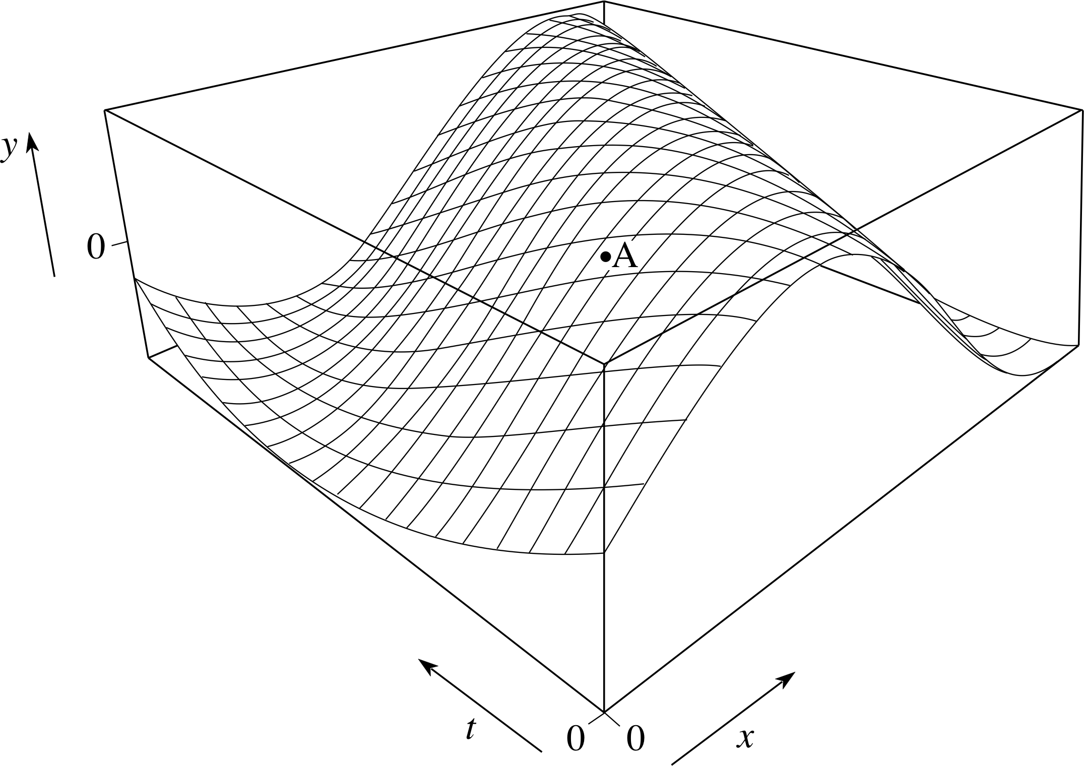
Figure 5 On the three–dimensional graph of a function of two variables there are generally many different gradients and many different derivatives at a single point.
You can see this in Figure 5, which you may, if you wish, regard as an enlargement of a small part of Figure 3. At the point marked A there is a gradient and hence a derivative in the x–direction, but there is also a gradient and a derivative in the t–direction, and in every other direction between those two. In discussing the gradient of the string at A (or B) what we are really interested in is the gradient in the x–direction at a particular time, and hence the derivative of y with respect to x while t is held constant.
This kind of derivative is called a partial derivative, and is represented by the symbol $\dfrac{\partial y}{\partial x}$ or, even more explicitly, $\left(\dfrac{\partial y}{\partial x}\right)_t$. i
So, using the partial derivative notation we can write the y–component of the total force on the segment at any time t:
Fy(A) + Fy(B) = FT(tan ϕ − tan θ)
as$F_y(A) + F_y(B) = F_{\rm T}\left(\dfrac{\partial y}{\partial x}(B)-\dfrac{\partial y}{\partial x}∂y(A)\right)$(10)
In a moment we will substitute this expression into Newton’s second law, but first we pause for a mathematical aside that tries to clarify the nature of these important partial derivatives.
Mathematical aside When dealing with a function of one variable, such as y = g (x), we can define its derivative (provided it exists) at any value of x by
$\displaystyle \dfrac{dy}{dx} = \lim_{h\to0}{\left[\dfrac{g(x+h)-g(x)}{h}\right]}$
Using this definition (or rules derived from it) we can easily find the derivative of a wide variety of simple functions. For example, if a, b, c, A are all constants:
ify = ax3then $\dfrac{dy}{dx} = 3ax^2$
ify = A sin(bx)then $\dfrac{dy}{dx} = Ab\cos(bx$) i
ify = A sin(c − bx) then $\dfrac{dy}{dx} = -Ab\cos(c-bx)$
Since the derivative dy/dx is itself a function of x, we may take its derivative, thus defining the second derivative:
$\dfrac{d^2y}{dx^2} = \dfrac{d}{dx}\left(\dfrac{dy}{dx}\right)$
In a similar way, when dealing with a function of two variables such as y = f (x, t) we can define the partial
$\displaystyle \dfrac{\partial y}{\partial x} = \lim_{h\to0}{\left[\dfrac{f(x+h,t)-f(x,t)}{h}\right]}$(11)
$\displaystyle \dfrac{\partial y}{\partial t} = \lim_{h\to0}{\left[\dfrac{f(x,t+h)-f(x,t)}{h}\right]}$(12)
Using these definitions we can easily find the partial derivatives of a range of functions of two variables, though in practice it is much easier to remember that in order to find a derivative such as ∂y/∂x all you have to do is to treat t as a constant and then proceed as you would when dealing with a function of x alone.
Thus, if a, b, A, k and ω are all constants:
if y = at3x2 then $\dfrac{\partial y}{\partial x} = 2at^3x\quad\text{and}\quad\dfrac{\partial y}{\partial t} = 3at^2x^2$
if y = A sin(kx − ωt) then $\dfrac{\partial y}{\partial x} = Ak\cos(kx\omega t)\quad\text{and}\quad\dfrac{\partial y}{\partial t} = -A\omega\cos(kx\omega t)$
Since the partial derivatives are also functions of two variables we may define the second_derivativesecond partial derivatives:
$\dfrac{\partial^2y}{\partial x^2} = \dfrac{\partial}{\partial x}\left(\dfrac{\partial y}{\partial x}\right),\quad\dfrac{\partial^2y}{\partial t^2} = \dfrac{\partial}{\partial t}\left(\dfrac{\partial y}{\partial t}\right)\quad\text{and}\quad\dfrac{\partial^2y}{\partial x\partial t} = \dfrac{\partial}{\partial x}\left(\dfrac{\partial y}{\partial t}\right)$
Question T4
Work out $\dfrac{\partial y}{\partial x},\dfrac{\partial y}{\partial t},\dfrac{\partial^2y}{\partial x^2},\dfrac{\partial^2y}{\partial t^2}, \dfrac{\partial^2y}{\partial x\partial t}\;\text{and}\;\dfrac{\partial^2y}{\partial t\partial x}$, in the following cases:
(a) y = A sin(btx)
(b) y = at + bx2 + ctx2
In each case a, b and c are constants.
Answer T4
(a) When finding $\dfrac{\partial y}{\partial x}$, treat t as a constant, so
$\dfrac{\partial y}{\partial x} = Abt\cos(btx)\quad\text{and}\quad\dfrac{\partial^2y}{\partial x^2} = -Ab^2t^2\sin(bxt)$
When finding $\dfrac{\partial y}{\partial t}$, treat x as a constant, so
$\dfrac{\partial y}{\partial t} = Abx\cos(btx)\quad\text{and}\quad\dfrac{\partial^2y}{\partial t^2} = -Ab^2x^2\sin(bxt)$
Also,$\dfrac{\partial^2y}{\partial x\partial t} = \dfrac{\partial}{\partial x}\dfrac{\partial y}{\partial t} = Ab\cos(bxt) - Ab^2xt\sin(bxt)$
$\phantom{\dfrac{\partial^2y}{\partial x\partial t} }= \dfrac{\partial}{\partial t}\dfrac{\partial y}{\partial x} = \dfrac{\partial^2y}{\partial t\partial x}$
(b) $\dfrac{\partial y}{\partial x} = 2bx + 2ctx,\;\dfrac{\partial^2y}{\partial x^2} = 2b + 2ct,\;\dfrac{\partial y}{\partial t} = a + cx^2,\;\dfrac{\partial^2y}{\partial t^2} = 0,\;\dfrac{\partial^2y}{\partial x\partial t} = 2cx = \dfrac{\partial^2y}{\partial t\partial x}$
$\dfrac{\partial^2y}{\partial x\partial t} = \dfrac{\partial^2y}{\partial t\partial x}$ for any function f (x, t) provided that it is continuous and differentiable.
Returning to our small segment of string, now that we know the y–component of force on the string we can use Newton’s second law to relate it to the y–component of the acceleration. Thus:
$F_{\rm T}\left(\dfrac{\partial y}{\partial x}({\rm B}) - \dfrac{\partial y}{\partial x}({\rm A})\right) = ma_y$(13)
where m is the mass of the segment and ay is its component of acceleration in the y–direction. If we define the mass per unit length of the string (the linear mass density) to be μ, then the mass of our string segment will be μ∆l, which we will take to be approximately equal to μ∆x. In principle ay should be the acceleration of the centre of mass of the string, but we will assume that the segment is sufficiently small that this acceleration is approximately equal to the acceleration of end A, so we can write:
$a_y \approx \dfrac{\partial^2y}{\partial t^2}({\rm A})$(14)
where the approximation will become increasingly accurate as the length of the segment is reduced.
It follows from Equations 13 and 14, together with the relation m = μ∆x, that:
$F_{\rm T}\left(\dfrac{\partial y}{\partial x}({\rm B}) - \dfrac{\partial y}{\partial x}({\rm A})\right) \approx \mu\Delta x\dfrac{\partial^2 y}{\partial t^2}({\rm A})$
i.e.$\dfrac{1}{\Delta x}\left(\dfrac{\partial y}{\partial x}({\rm B}) - \dfrac{\partial y}{\partial x}({\rm A})\right) \approx \dfrac{\mu}{F_{\rm T}}\dfrac{\partial^2 y}{\partial t^2}({\rm A})$
In the limit where the length of the segment becomes vanishingly small this approximation will become an equality, so we may write:
$\displaystyle \lim_{\Delta x\to0}\left[\dfrac{1}{\Delta x}\left(\dfrac{\partial y}{\partial x}({\rm B}) - \dfrac{\partial y}{\partial x}({\rm A})\right)\right] = \dfrac{\mu}{F_{\rm T}}\dfrac{\partial^2 y}{\partial t^2}({\rm A})$
Now, if we remember that both y and ∂y/∂x are actually functions of x and t, so that the segment ends A and B should really be specified in terms of a position and a time, as in (x, t) for A, and (x + ∆x, t) for B, we can rewrite this last relation as:
$\displaystyle \lim_{\Delta x\to0}\left[\dfrac{1}{\Delta x}\left(\dfrac{\partial y}{\partial x}(x+\Delta x,t) - \dfrac{\partial y}{\partial x}(x,t)\right)\right] = \dfrac{\mu}{F_{\rm T}}\dfrac{\partial^2 y}{\partial t^2}(x,t)$
The significance of this step is that it allows us to see that the term on the left–hand side is just the partial derivative with respect to x of ∂y/∂x (compare with Equation 11),
$\displaystyle \dfrac{\partial y}{\partial x} = \lim_{h\to0}{\left[\dfrac{f(x+h,t)-f(x,t)}{h}\right]}$(Eqn 11)
In other words the left–hand side is the second_derivativesecond partial derivatives of y with respect to x. Thus the transverse displacement y (x, t) must satisfy the equation
$\dfrac{\partial^2y}{\partial x^2} = \dfrac{\mu}{F_{\rm T}}\dfrac{\partial y}{\partial t^2}$(15) i
Equation 15 is of great importance.
Although we have only derived it at a certain point, defined by x and t, there was nothing special about those coordinates, so it must be true at any point x and any time t. Moreover, the same equation can be obtained even if we relax some of the simplifying assumptions we made earlier, so it actually represents a very general condition that the transverse displacement must satisfy. Mathematically it may be described as a linear_second_order_differential_equationlinear second-order partial differential equation, i and is one form of the wave equation that will be discussed shortly. By identifying Equation 15 as a special case of the wave equation we will soon be able to relate the phase speed of waves on a string to μ and FT, the linear mass density and tension magnitude of the string.
The derivation of Equation 15 is typical of the derivations of the wave equations for other physical systems. We start from the basic physics in a system, analyse the forces that result from a deviation from equilibrium, make approximations based upon those deviations being small enough, and come up with a partial differential equation which describes the motion in the system. If the approximations of smallness are not made, we will generally end up with a non_linear_differential_equationnon–linear equation, and much more complicated mathematical and physical behaviour; we will not deal with these in FLAP.
2.6 The speed of waves on a string
We now have an equation of motion (Equation 15) based on the physics of a string under tension. To verify that sinusoidal periodic waves of the kind described by Equations 4–8:
y = A sin[k (x − υt)](Eqn 4)
y = A sin(kx − ωt)(Eqn 5)
y = A sin[2π (σx − ft)](Eqn 6)
$y = A\sin\left[2\pi\left(\dfrac x\lambda - ft\right)\right]$(Eqn 7)
$y = A\sin\left[2\pi\left(\dfrac x\lambda - \dfrac tT\right)\right]$(Eqn 8)
satisfy Equation 15, we need to determine the relevant partial derivatives of the sine function and show that they satisfy the equation of motion.
According to Equation 5, the transverse displacement y of a sinusoidal wave is given by
y = A sin(kx − ωt)(Eqn 5)
so$\dfrac{\partial y}{\partial x} = Ak\cos(kx\omega t)$
and$\dfrac{\partial^2y}{\partial x^2} = \dfrac{\partial}{\partial x}\left(\dfrac{\partial y}{\partial x}\right) = -Ak^2\sin(kx\omega t)$
thus$\dfrac{\partial^2y}{\partial x^2} = -k^2y$(16)
✦ Calculate the second partial derivative of y with respect to t.
✧ The first derivative is calculated as above, but we obtain an extra minus sign because the ωt term is preceded by a minus sign:
$\dfrac{\partial y}{\partial t} = -A\omega\cos(kx-\omega t)$
and$\dfrac{\partial^2y}{\partial t^2} = \dfrac{\partial}{\partial t}\left(\dfrac{\partial y}{\partial t}\right) = -A\omega^2\sin(kx-\omega t)$
thus$\dfrac{\partial^2y}{\partial t^2} =-\omega^2y$(17)
Substituting Equations 16 and 17,
$\dfrac{\partial^2y}{\partial x^2} = -k^2y$(Eqn 16)
$\dfrac{\partial^2y}{\partial t^2} = -\omega^2y$(Eqn 16)
into the equation of motion (Equation 15),
$\dfrac{\partial^2y}{\partial x^2} = \dfrac{\mu}{F_{\rm T}}\dfrac{\partial y}{\partial t^2}$(Eqn 15)
we obtain:
$-k^2y = -\dfrac{\mu}{F_{\rm T}}\omega^2y$
i.e.$\dfrac{k^2}{\omega^2} = \dfrac{\mu}{F_{\rm T}}$(18)
Thus, the sinusoidal waves described by Equation 5,
y = A sin(kx − ωt)(Eqn 5)
will satisfy Equation 15 provided $k/\omega = \sqrt{\mu/F_{\rm T}}$. However, according to Equation 9,
υ = ω/k(Eqn 9)
ω/k is just the speed of propagation υ (i.e. the phase speed) of the sinusoidal waves. Hence, Equation 18 implies:
$\upsilon = \sqrt{\dfrac{F_{\rm T}}{\mu}}$(19)
So we have found that the sine wave is a solution of the equation of motion for a string if the speed of propagation is given by the square root of the tension magnitude divided by the mass per unit length. This is an important result, because its general character will extend to waves on other media. Each physical system must be considered in its own right, but it is common to find that the propagation speed is given by an expression similar to Equation 19 with FT replaced by the magnitude of the force restoring the medium to its equilibrium position, and μ replaced by some parameter that characterizes the inertia in the system, i.e. the tendency of the medium to remain in a given state of motion.
Question T5
Determine the units of the expression $\sqrt{F_{\rm T}/\mu}$.
Answer T5
The units of FT are N, or kg m s−1; the units of μ are kg m−2.
The ratio then has the units (kg m s−2/kg m−1) = m2 s−2.
Finally, the units of the square root are (m2 s−2)1/2 = m s−1, which are the units of speed, as required.
Question T6
A wire has a linear mass density of 5.5 g m−1, and is under a tension of 500 N. What is the phase speed of transverse sinusoidal waves in this wire?
Answer T6
First we need to make the units consistent: μ = 5.5 g m−1 = 5.5 × 10⁻³ kg m−1. Then:
$\upsilon = \rm \sqrt{\dfrac{5\times10^2\,kg\,m\,s^{-2}}{5.5\times10^{-3}\,kg\,m^{-1}}} = \sqrt{9.09\times10^4\,m^2\,s^{-2}}$
i.e.υ = 302 m s−1 = 300 m s−1 (to two significant figures)
2.7 The energy of waves on a string
It was stated earlier that waves often involve the transfer of energy from place to place. This subsection is devoted to a discussion of the energy transferred by a wave on a string, but, as in the last subsection, some of the results are indicative of the behaviour of a wide variety of physical systems. As is usual for a mechanical system, the total energy of a wave on a string comprises kinetic energy and potential energy. The kinetic energy arises from the motion of the various parts of the string, while the potential energy arises from the work done by the restoring force acting on each element that departs from equilibrium. Up to this point, we have considered parts of the wave that are far enough away from the ends of the string that the length of the string is irrelevant. In order to continue doing this it is convenient to characterize the energy associated with the waves in terms of a linear energy density DE(x, t). This can be determined by measuring the total energy E associated with a short segment of string of length ∆l, centred on x at time t, and then determining the ratio E/∆l as ∆l becomes vanishingly small. In this way we can define DE(x, t) as the energy per unit length of the string at x and t, and we see that it can be measured in units of joules per metre (J m−1). i
Figure 4 A small segment of string and the forces that act on it due to the tension in the string. Tangents to the string, drawn at the end points A and B of the segment, make angles θ and ϕ with the positive x–axis. The angles in the figure are positive and large enough to be clearly seen, but in principle they might be negative and we shall assume that whatever their sign they are actually very small.
The kinetic energy contribution to DE(x, t) is fairly straightforward; the mass of the segment is μ∆x, and the velocity is ∂y/∂t, so the kinetic energy term is:
$\dfrac12\mu\Delta x\left(\dfrac{\partial y}{\partial t}\right)^2$
The potential energy contribution is more difficult to derive; here we will just quote the value, which is:
$\dfrac12F_{\rm T}\left(\dfrac{\partial y}{\partial t}\right)^2\Delta x$
To see that this is at least plausible, remember the discussion in Subsection 2.5 of the forces acting on a small segment, as shown in Figure 4. When y is at a maximum value, there are no forces acting on the segment, so it is not stretched, and the potential energy is zero. On the other hand, when y = 0, the slope of the curve is steepest, and the potential energy is a maximum.
Then this linear energy density can be expressed as:
$D_E(x,t) = \dfrac12\left[\mu\left(\dfrac{\partial y}{\partial t}\right)^2 + F_{\rm T}\left(\dfrac{\partial y}{\partial t}\right)^2\right]$(20)
The first term corresponds to the kinetic energy per unit length, or the linear kinetic energy density. The second term corresponds to the linear potential energy density.
This general expression is not very informative, so we will restrict our discussion to the case of sinusoidal waves. We calculated the required first derivatives in the preceding subsection, so we can substitute these directly into the energy density equation:
$D_E(x,t) = \dfrac12\left\{\mu\left[-A\omega\cos(kx-\omega t)\right]^2 + F_{\rm T}\left[Ak\cos(kx-\omega t)\right]^2\right\}$
so$D_E(x,t) = \dfrac12 A^2(\mu\omega^2 + F_{\rm T}k^2)\cos^2(kx-\omega t)$(21)
It is interesting to compare the linear energy density at a point on the string with the energy of a simple harmonic oscillator. In the latter case the total energy of the oscillator is constant, but its form fluctuates between kinetic energy and potential energy. In the case of the wave on a string, the linear energy density is itself a travelling wave, so energy is being carried along the string and the energy density at any fixed point (i.e. at any fixed value of x) oscillates with time. The kinetic and potential energy densities have the same functional dependence on x and t, so their maxima and minima occur simultaneously at any given point.
Using Equation 18,
$\dfrac{k^2}{\omega^2} = \dfrac{\mu}{F_{\rm T}}$(Eqn 18)
we can see that μω2 = FTk2, so we can rewrite Equation 21 more compactly as:
DE(x, t) = μω2A2 cos2(kx − ωt)(22)
We now see that the magnitude of the linear energy density is proportional to the square of both the amplitude and the frequency of the wave. This makes good physical sense: if you were generating the waves by shaking one end of the string you would have to shake more vigorously and supply more energy if you wanted to increase either the amplitude or the frequency, or both. i
The energy density of Equation 22 is clearly a periodic wave, but the presence of the square of the cosine function makes it difficult to determine its wave parameters. However, if we use the following trigonometric identity i:
$\cos^2\theta = \dfrac{1 + \cos(2\theta)}{2}$
we can rewrite the energy density as:
$D_E(x,t) = \dfrac{\mu\omega^2A^2}{2}\left[1 + \cos(2kx - 2\omega t)\right]$
We can now introduce some new constants, $D_0 = \dfrac{\mu\omega^2A^2}{2}$, kE = 2k and ωE = 2ω, and use them to write:
DE(x, t) = D0[1 + cos(kEx − ωEt)](23) i
This equation shows that the linear energy density has a constant average value, D0, about which it fluctuates in a wave–like way, though it never becomes negative. This wave–like fluctuation in the energy density has an angular wavenumber kE which is twice that of the original displacement wave, and an angular frequency ωE which is twice that of the original. This leads to a wavelength λE and a period TE which are half the original values, resulting from the fact that the energy density does not depend on the signs of the transverse velocity and transverse displacement. At a fixed value of x, the linear energy density wave passes through a maximum whenever the displacement is zero, and the instantaneous energy density minima occur when the displacement is at the extreme in the positive or negative direction. This is another fundamental characteristic of sinusoidal waves.
Question T7
Sketch the profile of the linear energy density wave at a fixed time t1, along with the profile of the corresponding displacement wave at the same time. Show explicitly the relationships between the wavelengths of these two waves.
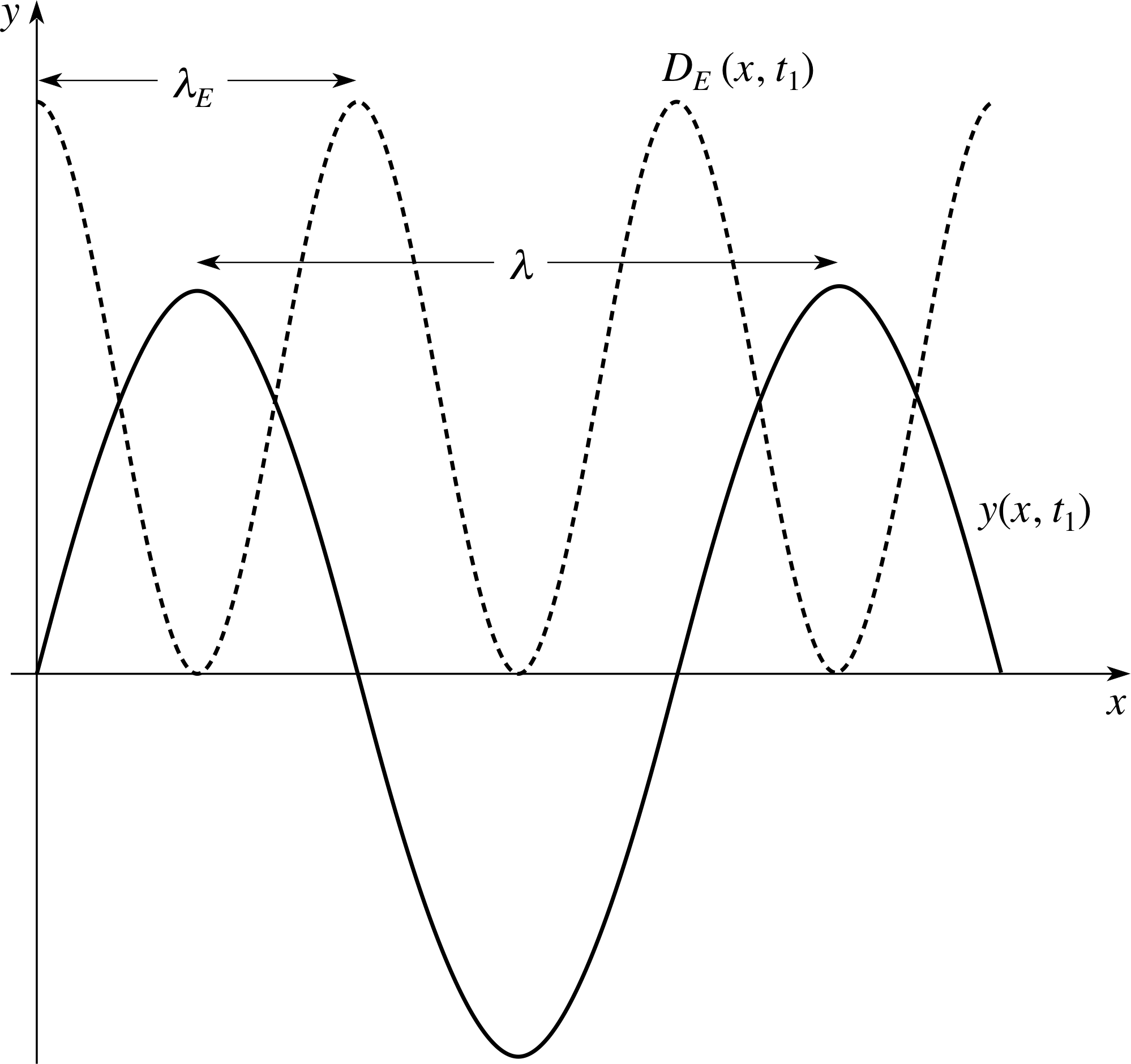
Figure 18 See Answer T7.
Answer T7
The original sine wave has zeros when (kx − ωt1) = 0, π, and 2π. The argument of the cosine function in the energy density wave will be 0, 2π, and 4π at those points, which produces maxima in the energy density wave.
When (kx − ωt1) = π /2 and 5π/2, the displacement wave exhibits maxima, while the energy cosine function takes the value −1, which makes the energy density zero. The sketch in Figure 18 illustrates this at t = t1.
2.8 The generalized wave equation
In Subsection 2.5 we obtained the equation of motion for waves on a string; the linear second–order partial differential equation
$\dfrac{\partial^2y}{\partial x^2} = \dfrac{\mu}{F_{\rm T}}\dfrac{\partial y}{\partial t^2}$(Eqn 15)
and in Subsection 2.6 we showed that sinusoidal functions y (x, t) = sin(kx − ωt) satisfying this equation described waves that propagated with phase speed
$\upsilon = \sqrt{\dfrac{F_{\rm T}}{\mu}}$(Eqn 19)
Combining these two results we obtain the equation
$\dfrac{\partial^2y}{\partial x^2} = \dfrac{1}{\upsilon^2}\dfrac{\partial y}{\partial t^2}$(24)
Now, although we have arrived at Equation 24 by considering the special case of sinusoidal waves, it is in fact a more general condition, the validity of which extends far beyond the sinusoidal waves we have emphasized. Equation 24 is known as the (simple) wave equation for waves on a string. i) Any wave that travels with constant speed and unchanging shape, will be described by a function of the form y = f (kx ± ωt), and will satisfy the wave equation.
Wave equations are not restricted to waves on strings. Similar equations may be obtained for other physical systems that support transverse waves travelling with constant speed and unchanging shape. In the general case, the dependent variable that is the subject of the equation will not necessarily be a transverse displacement y, though it will describe some kind of ‘transverse’ departure from equilibrium. If we represent this generalized disturbance by the quantity Ψ (x, t), i then it must satisfy the generalized one–dimensional (motion along x) wave equation:
$\dfrac{\partial^2{\it\Psi}}{\partial x^2} = \dfrac{1}{\upsilon^2}\dfrac{\partial{\it\Psi}}{\partial t^2}$(25)
In any particular case the speed of wave propagation υ will always be determined by the physics of the system, but in the case of mechanical systems it will generally be given by the square root of the ratio of a restoring force parameter to the inertial parameter, just as it was in Equation 19 for waves on a string.
2.9 Summary of Section 2
We have covered a great deal of material in this section on transverse travelling waves, and it is worth reviewing the basic ideas at this point. We first considered the physical description of transverse travelling waves. We saw that it is the disturbance, a departure from equilibrium that propagates, not some part of the medium that carries that disturbance. Having that as our basis, we found a general mathematical description of a wave on a string propagating in either direction in one dimension [y = f (x ± υt)]. We then introduced the idea of a periodic wave characterized by a wavelength and a period, and chose to concentrate on the particularly important case of a sinusoidal wave (y = A sin(kx − ωt)). Here we explained the significance of, and relationship between the fundamental parameters υ, T, f, ω, λ, σ and k. We next looked in greater detail at the physics of transverse waves on a string, and saw how the restoring force of the unbalanced tension led to a second–order linear partial differential equation which described the motion of the system. We then showed that the sinusoidal waves we had previously looked at were solutions of this equation, provided that locations of fixed transverse displacement y (and hence fixed phase (kx − ωt)) propagated with a unique (phase) speed that was simply related to the tension and linear mass density of the string. We also developed the concept of the linear energy density of the wave on a string, and showed for the standard case of sinusoidal waves, the energy density was also a wave, with the same phase speed, but half the wavelength and twice the frequency of the original transverse displacement wave. Finally, we considered the (simple) wave equation for waves on a string and its generalization to cover a wide class of transverse waves that travel in one dimension with constant speed and unchanging shape.
3 Superposition and interference
3.1 The superposition principle
The property of linearity possessed by the simple wave equation means that if Ψ1(x, t) and Ψ2(x, t) are solutions of the equation then a linear combination of those solutions, i.e. any expression of the form Ψ(x, t) = aΨ1(x, t) + bΨ2(x, t), where a and b are any numerical constants, will also be a solution. A consequence of this is the following principle:
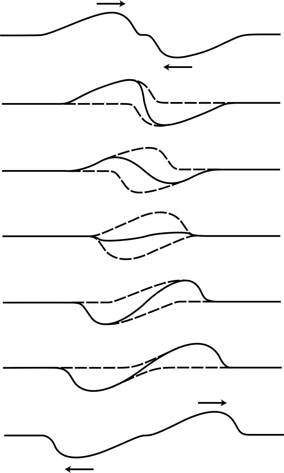
Figure 6 The superposition principle applied to two pulses moving toward each other, shown at seven successive times (moving from top to bottom). Where the pulses overlap, the dashed lines indicate the shape of the individual pulses, while the solid line is the actual displacement profile of the string.
The superposition principle
If two or more waves meet in a region of space, then at each instant of time the net disturbance they cause at any point is equal to the sum of the disturbances caused by each of the waves individually.
This principle may be applied to any system in which the waves of interest are described by linear equations. In those cases where it can be applied, the superposition principle enormously simplifies the study of waves, since it allows us to treat complicated waves as a superposition (i.e. a sum) of simple waves that are easier to analyse. Ultimately, it allows us to describe any periodic wave in terms of the familiar sinusoidal waves.
What does the superposition principle mean physically? It implies, for example, that when two separate pulses travelling in opposite directions on a single string meet in some shared region of the string, as shown in Figure 6, then we can find their combined effect at any place and time by simply adding the separate contributions (displacements) from the two pulses at that place and time. What happens after the pulses pass through the shared region? They regain their original shapes and continue moving as before, being individually unchanged by the passage through the shared region.
Another way of regarding the superposition principle is as a requirement that the presence of a wave at a point in a medium should not change the physical properties of the medium at that point. If the passage of a wave along a string caused an appreciable change in the tension, then a second wave on the same string would experience a ‘different’ medium (with a different phase speed), and the two waves could be not simply added together.
Question T8
Two wave pulses travelling in opposite directions along a string are described by the following functions:
$y_1(x,t) = \dfrac{A}{\left[\left(\dfrac{bx-ct}{2}\right)^2+1\right]}\quad\text{and}\quad y_2(x,t) = \dfrac{A}{\left[\left(\dfrac{bx+ct}{2}\right)^2+1\right]}$
If A = 50 mm, b = 0.1 mm−1 and c = 2 s−1, sketch the profile of the resultant pulse at t = 1 s.
(You will probably find it convenient to consider values of x in the range −20 cm to +20 cm.)
Answer T8
When t = 1 s, we need to sketch the function:
$y = \dfrac{50\,{\rm mm}}{\left\{\left[\dfrac{(0.1x/{\rm mm})-2}{2}\right]^2+1\right\}} + \dfrac{50\,{\rm mm}}{\left\{\left[\dfrac{(0.1x/{\rm mm})+2}{2}\right]^2+1\right\}}$
After a little algebra, and converting units from mm to cm:
$y = 20\,{\rm cm}\left\{\left[\dfrac{1}{(x/{\rm cm})^2-4(x/{\rm cm})+8}\right] + \left[\dfrac{1}{(x/{\rm cm})^2+4(x/{\rm cm})+8}\right]\right\}$
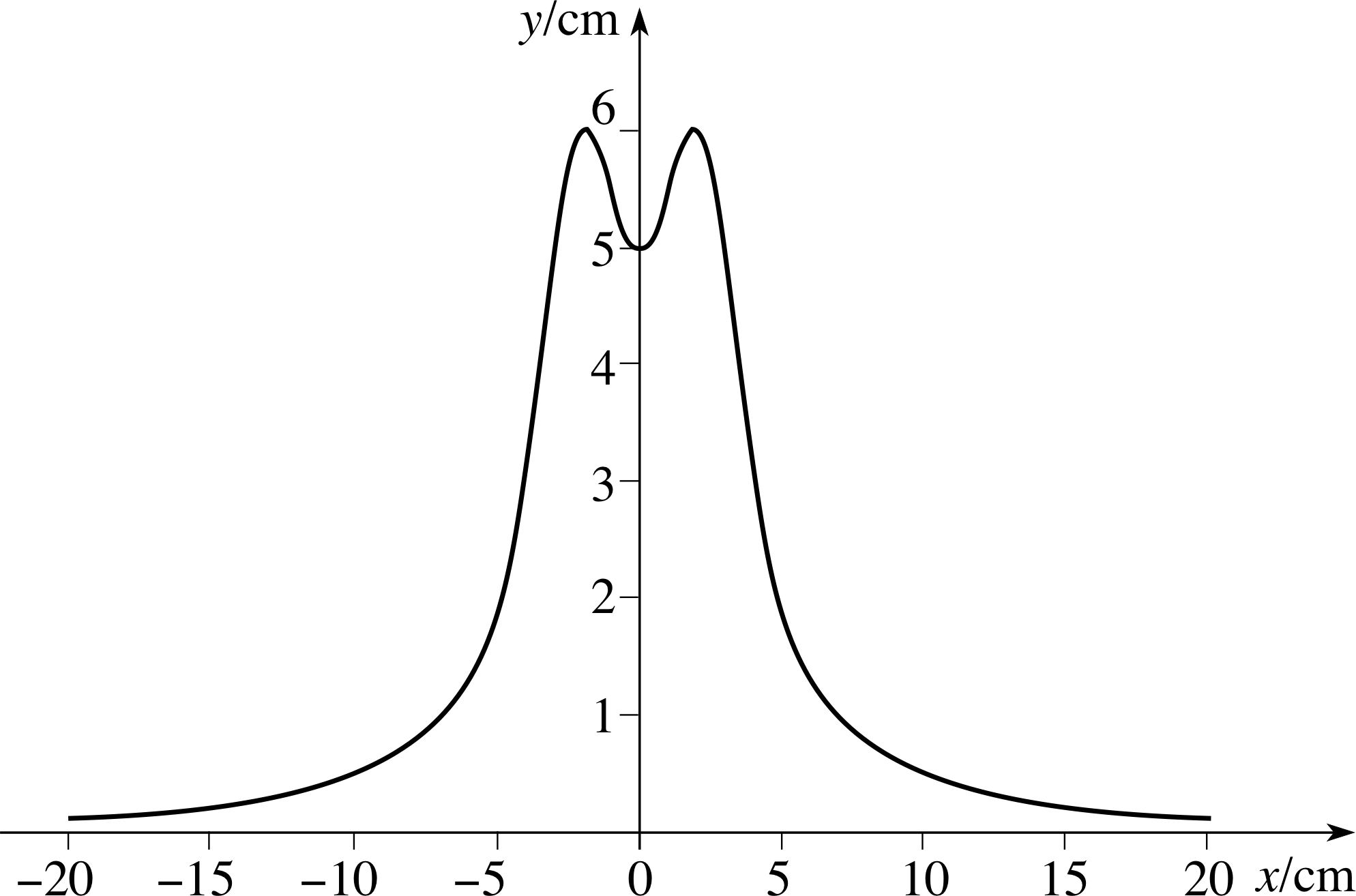
Figure 19 See Answer T8.
The sketch is shown in Figure 19 for values of x between −20 cm and +20 cm.
3.2 Interference
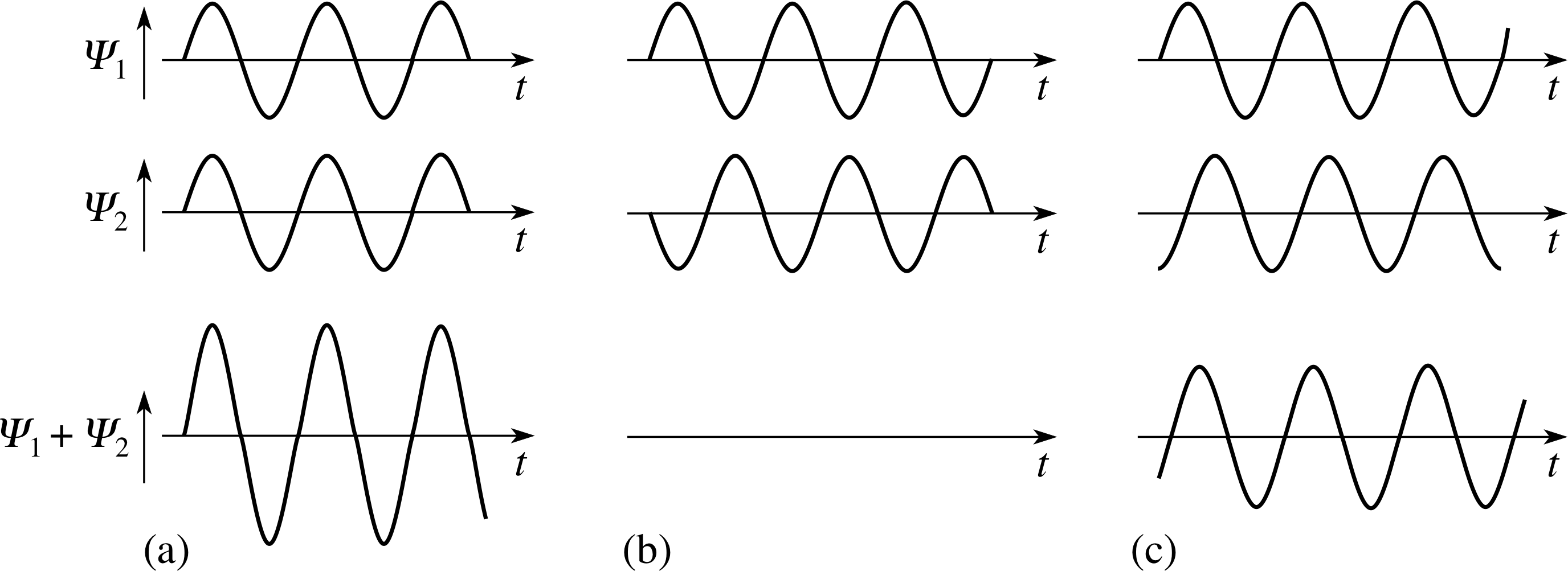
Figure 7 Wave forms at a point arising from the interference of two waves of equal amplitude and frequency passing through that point. (a) Fully constructive interference, showing the doubling of the amplitude. (b) Fully destructive interference, showing the cancellation of amplitudes. (c) The intermediate case where partial addition of the amplitude occurs.
One of the most important consequences of the superposition principle is the phenomenon of interference, iwhich allows periodic waves travelling along a line to combine and produce some other wave along that line, as shown in Figure 7. If the waves Ψ1(x, t) and Ψ2(x, t) that are being combined have the property that at a certain point they both cause the maximum disturbance at the same time (Figure 7a) then they are said to be in phase at that point and they will cause totally constructive interference at that point. As a result the waves will reinforce one another at the point in question and the amplitude of the resulting disturbance will be equal to the sum of the individual amplitudes at that point.
In contrast, if the waves are completely out of phase (i.e. in antiphase) at a point their effects will cancel at that point and the result will be totally destructive interference, as shown in Figure 7b.
More generally, waves arriving at a single point will not be completely in phase, nor completely out of phase, and the resulting disturbance will then be somewhere between the extremes, as shown in Figure 7c.
✦ If the sinusoidal wave forms shown in Figure 7b had different amplitudes A1 and A2 (with A1 greater than A2), how would the superposed waveform be changed?
✧ It would have been sinusoidal, in phase with the wave form of amplitude A1, and of amplitude A1 − A2.
Recalling that the instantaneous energy density carried by a wave (Equation 22),
DE(x, t) = μω2A2 cos2(kx − ωt)(Eqn 22)
is proportional to the square of the amplitude, destructive superposition has an amazing consequence. Two waves, each of which individually carries energy at a point in space and time, can add together to produce a resultant wave which carries no energy at that point.i
The superposition principle is a fundamental characteristic of systems that obey a linear differential equation. On the other hand, if a system is non-linear, then the superposition principle will break down, and the analysis becomes much more complicated and specialized.
3.3 Wave groups and group speed
An important case of superposition is that which arises when two or more travelling waves moving in the same direction with closely similar frequencies are combined.
Question T9
Use the trigonometric identity
$\sin(\alpha) + \sin(\beta) = 2\sin\left(\dfrac{\alpha+\beta}{2}\right)\cos\left(\dfrac{\alpha-\beta}{2}\right)$
to find the wave that results from the superposition of
y1 = A sin(kx − ωt) and y2 = Asin[(k + ∆k)x − (ω + ∆ω)t]
where ∆ω and ∆k are small positive quantities. Assuming ∆k is about one–tenth of k, sketch the profile of the combined wave at t = 0, over the range from x = 0 to x = 20 (2π/k), i.e. over about 20 ‘wavelengths’.
[Hint: don’t try plotting this profile point by point – it will take far too long. Treat it as a product of two factors, sketch their graphs very roughly, then think about what the graph of their product must look like before sketching it equally roughly.]
Answer T9
$y = y_1 +y_2 = 2A\sin\left[\left(\dfrac{2k+\Delta k}{2}\right)x - \left(\dfrac{2\omega+\Delta\omega}{2}\right)t\right]\times\cos\left[\left(\dfrac{\Delta k}{2}\right)x - \left(\dfrac{\Delta \omega}{2}\right)t\right]$
When sketching the graph of this function at t = 0 (or any other time) it is best regarded as a product of two factors as in:
$y = 2A\cos\left[\left(\dfrac{\Delta k}{2}\right)x - \left(\dfrac{\Delta \omega}{2}\right)t\right]\times\sin\left[\left(\dfrac{2k+\Delta k}{2}\right)x - \left(\dfrac{2\omega+\Delta\omega}{2}\right)t\right]$
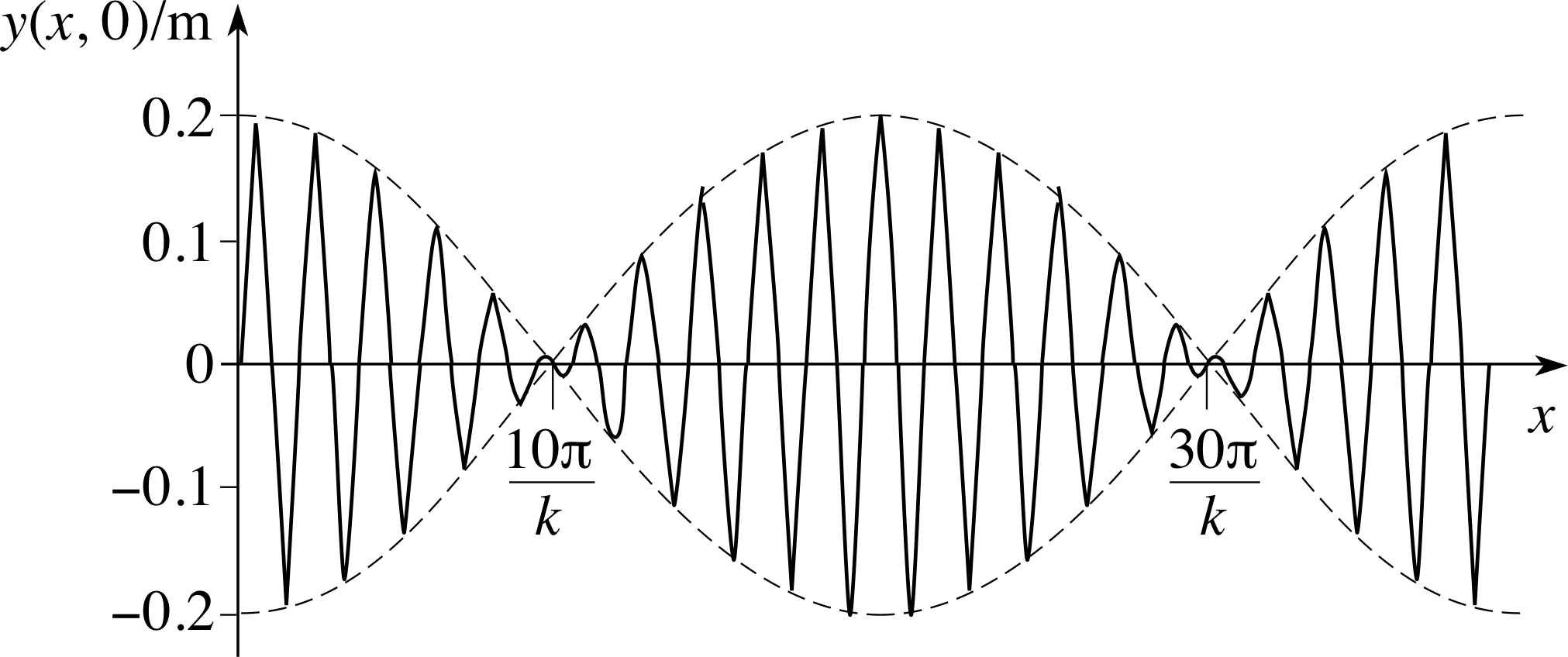
Figure 20 See Answer T9.
Both of the bracketed expressions represents a wave, though the first will have a much longer wavelength (4π/∆k), and usually a lower speed (∆ω/∆k), than the second. In view of this, it is better to regard the first expression as a moving ‘envelope’ that determines the effective amplitude of the shorter wavelength sine waves at any particular place and time.
The required wave profile at t = 0 of a wave group composed of two sinusoidal waves of slightly different (angular) frequencies ω and ω + ∆ω is shown in Figure 20. The instantaneous shape of the moving envelope that plays such a major part in shaping the profile is shown by a dashed line.
If the waves described in this question satisfy the simple wave equation (Equation 25),
$\dfrac{\partial^2{\it\Psi}}{\partial x^2} = \dfrac{1}{\upsilon^2}\dfrac{\partial{\it\Psi}}{\partial t^2}$(Eqn 25)
then they must both travel with the same speed i, hence
υ = ω/k = (2ω + ∆ω)/(2k + ∆k)
and the profile shown in the answer (Figure 20) to Question T9 will also travel at that speed. However, in many important situations, such as that of waves on the surface of a pond, or even waves on a string if we admit that the passage of a wave really does affect the tension to some extent, waves of different (angular) frequency actually travel at different speeds. This phenomenon, the frequency dependence of the propagation speed, is known as dispersion. Amongst other things it means that travelling waves of slightly different frequency that are initially in phase at some point will become progressively out of phase at that point as time passes.
The superposition of waves described in Question T9 and illustrated in Figure 20 has the form
$y = \left\{2A\cos\left[\left(\dfrac{\Delta k}{2}\right)x-\left(\dfrac{\Delta\omega}{2}\right)t\right]\right\}\times\left\{2A\sin\left[\left(\dfrac{2k+\Delta k}{2}\right)x-\left(\dfrac{2\omega+\Delta\omega}{2}\right)t\right]\right\}$
Figure 20 See Answer T9.
Each of the bracketed expressions represents a wave. The first, with a very much longer wavelength than the second, moves with a speed υg = ∆ω/∆k, while the second, with a wavelength much the same as the two original components, has a different speed υp = (2ω + ∆ω)/(2k + ∆k). The difference between the wavelengths of the two terms is so marked that it is better to regard the first term as providing the overall shape, or ‘envelope’ of the second at any particular place and time.
In Figure 20 the envelope is shown as the dashed line, which controls or ‘modulates’ the amplitude of the short wavelength wave. The overall disturbance is called a wave group; it moves at a speed υg, which is called the group speed, and the waves appearing to move within the envelope move with the phase speed υp.
4 Standing waves on a string
4.1 Reflection of travelling waves at a boundary
So far, we have considered travelling waves far away from any boundaries that might affect their motion. We now want to look at what happens when one of these waves is incident on a boundary. The physical situation we want to consider first is a wave pulse propagating along a string which reaches a position at which the string is attached to something else. The resulting behaviour of the wave depends on what happens physically at that point of attachment. This is characterized mathematically by the boundary conditions, which are the requirements imposed on the values of the wave y (x, t), and, possibly, its derivatives, at the boundary. i We will start by examining the case in which the string is attached to a fixed object, such as a wall.
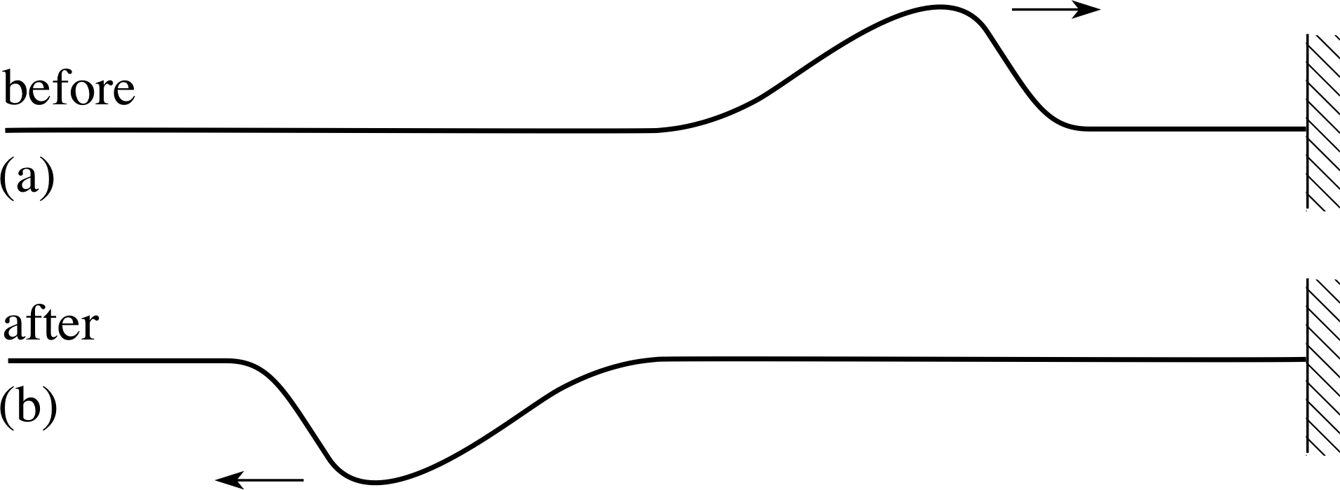
Figure 8 (a) A wave pulse travels in the +x–direction toward a wall. (b) After reflection, a wave pulse travels back in the −x–direction, with the same shape and amplitude, but opposite displacement.
Consider the pulse shown in Figure 8a. In this particular case the boundary condition implies that the transverse displacement at the wall must be zero. When the pulse reaches the wall, the moving string will exert an upward force on the wall. However, the wall is rigid and immovable, so it remains motionless. Consequently no mechanical energy will be transferred to the wall. In accordance with Newton’s third law, the wall will exert a downward reaction force on the string and this will cause a reflected pulse to travel away from the wall in the −x–direction. This reflected pulse will carry away all the incident energy, so it must have the same amplitude as the incident pulse, but its displacement will be negative where that of the original pulse was positive. This is indicated in Figure 8b.
Question T10
A wave pulse travelling towards a rigid wall at x = 0 starts its journey at t = −T and is described by yincident = A exp[−(bx + at)2],where a and b are positive constants. The pulse arrives at the wall at t = 0 and is then reflected. Write down an expression representing the reflected pulse at any (positive) time t.
Answer T10
Since a and b are positive, the bx + at term indicates motion in the −x–direction at speed υ = a/b. (A fixed value of the phase, bx + at = constant, corresponds to decreasing values of x as t increases.) Since the pulse arrives at x = 0 at t = 0, it must initially be travelling along the positive part of the x–axis towards x = 0. At any positive time t = τ the transverse displacement of the reflected pulse at a given position x will be equal in magnitude but opposite in sign to that of the incident pulse at the same position at t = −τ. Thus, yreflected(x, t) = −yincident(x, −t).
It follows that:
yreflected(x, t) = −A exp[−(bx − at)2]
Note that the original pulse was moving in the −x–direction but the reflected pulse moves in the +x–direction.
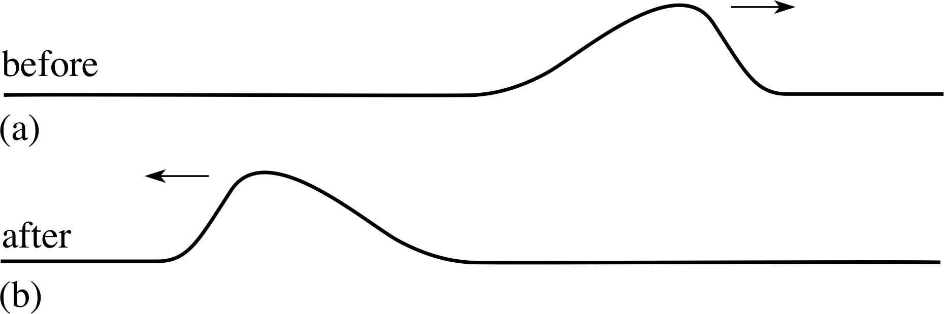
Figure 9 (a) A wave pulse travelling toward a freely moving boundary. (b) The reflected pulse.
If in place of a rigid wall the string was attached to a massless, frictionless ring on a pole, it would have a free end at the boundary rather than a fixed end. Under these conditions there will still be a reflected wave but its nature will be quite different from that of a reflection from a wall. This is indicated in after Figure 9, where you can see that the transverse displacement of the reflected pulse does not suffer the sign reversal that occurred in the case of a rigid wall.
In the more general case in which we consider the boundary to be between two different media (such as strings with different mass densities), the boundary conditions can be more general. The behaviour of the wave will be more complicated, with part of the wave being reflected (either with or without inversion, depending on the physical conditions) and part being transmitted.
4.2 Production of standing waves by superposition
We now consider the combined effect of two periodic sinusoidal waves, travelling in opposite directions along a string. We will assume that the two travelling waves have equal amplitude and the same frequency (and hence the same wavelength). We will write the travelling waves as:
y+ = A sin(kx − ωt) and y− = A sin(kx + ωt)(26)
The total wave, by the principle of superposition, will be just the sum:
y = y+ + y− = A sin(kx − ωt) + A sin(kx + ωt)(27)
By making use of the trigonometric identity sin(α + β) = sin(α) cos(β) + cos(α) sin(β) and the symmetry relations sin(−α) = −sin(α) and cos(−α) = cos(α) we can rewrite Equation 27 as:
y = A sin(kx) cos(ωt) − A cos(kx) sin(ωt) + A sin(kx) cos(ωt) + A cos(kx) sin(ωt)
i.e.y = 2A cos(ωt) sin(kx)(28)
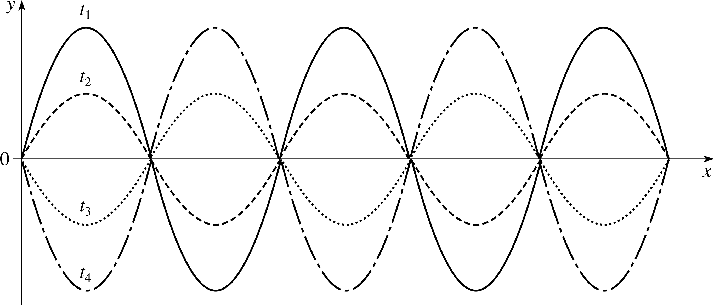
Figure 10 A standing wave on a string can be represented as a superposition of oppositely moving travelling waves, but the standing wave itself shows no tendency to move to the right or to the left. Consequently, such waves do not transfer energy from place wave changes with time as to place. t1 < t2 < t3 < t4.
This function is a product of a cosine function involving time and a sine function involving position, rather than a single function of the combination of position and time (e.g. kx ± ωt).
This change means that the combined disturbance is not a travelling wave. Such a disturbance is called a standing wave, or a stationary wave.
The profile of the standing Figure 10 indicates, but the wave has no tendency to move to the right or to the left. i
Question T11
Suppose our original waves in the above passage were described by cosine functions, i.e. y+ = Acos(kx − ωt) and y− = Acos(kx + ωt). What would be the resulting form for y = y+ + y−? Would it be a standing wave?
[Note that cos(α + β) = cos(α) cos(β) − sin(α) sin(β).]
Answer T11
y = A [cos(kx) cos(ωt) + sin(kx) sin(ωt) + cos(kx) cos(ωt) − sin(kx) sin(ωt)]
i.e.y = 2A cos(ωt) cos(kx)
The separation of the dependence on x and t means that this will be a standing wave.
4.3 Nodes and antinodes
As shown in Figure 10, the characteristic feature of standing waves is the development of a changing but non–progressing (or stationary) wave profile. One prominent feature of this is the existence of positions where no motion occurs at any time. Unlike travelling sinusoidal waves, where the displacement at each position undergoes simple harmonic oscillations of a uniform amplitude, in standing waves there are positions of complete rest at regular intervals. These positions are called node_in_a_standing_wavenodes.
y = 2A cos(ωt) sin(kx)(Eqn 28)
In the standing wave described above we can see that the sine function, and hence the transverse displacement, will vanish at all times at any position x = xnodal where the argument of the sine function is a multiple of π, i.e. where kxnodal = 0, ±π, ±2π, ±3π, ... = nπ with n = 0, ±1, ±2, ... .
Equivalently, since k = 2π/λ, these nodal positions are given by:
$x_{\rm nodal} = \dfrac{\lambda}{2\pi}n\pi = \dfrac{n\lambda}{2}$(29)
This shows that the spacing of the nodes is just (λ/2). Note in Figure 10 that the string has displacements of opposite sign on opposite sides of each node. This is a fundamental characteristic of nodes and standing waves.
Halfway between these nodes, the oscillations in time produce the maximum amplitude variation. These points at which the maximum amplitude oscillations take place are called the antinodes.
The positions of the antinodes can be found by requiring the sine function to have its maximum values of ±1, and are given by:
$x_{\rm antinodal} = \left(n+\dfrac12\right)\dfrac{\lambda}{2}$ with n = 0, ±1, ±2, ...(30)
Question T12
Confirm that the above condition gives the correct positions for the antinodes.
Answer T12
The requirement for an antinode is that sin(kx) = ±1, which means that kxsinusoidal must be an odd multiple of π/2, which can be written (2n + 1)π/2.
Thus,$x_{\rm antinodal} = \dfrac{(2n + 1)\pi}{2k} = \dfrac{(2n + 1)\pi}{2\times(2\pi/\lambda)} = \dfrac{(2n + 1)\lambda}{4} = \dfrac{(n + 1/2)\lambda}{2}$
If we consider standing waves produced on a string of a given length l, which is rigidly fixed at its two ends, then we know that the boundary conditions at the ends of the string require that the displacement should be zero at those points. We will label the end positions as x = 0 and x = l. Then we must have:
y (0) = 0 and y (l) = 0
and sosin(k) = sin(kl) = 0
Thus, remembering that k = π/λ, we have here the condition that l = nλ/2, or that
λ = l/n(31)
(with n any non–zero whole number). In the general case of standing waves on an infinite string, the spacing of the nodes depended on the wavelength, but any wavelength was possible. For a string of finite length, the additional condition that both ends must be nodes produces a constraint on the wavelengths that can be sustained on the string. We will examine the consequences of this further in the next subsection.
4.4 Stringed musical instruments
Stringed musical instruments such as guitars, violins or pianos provide everyday examples of transverse standing waves. In all these cases, a mechanical impulse (a finger, pick, bow or hammer) creates a wave on the string, and the only components of the wave that last are those which represent possible standing waves on the string. Since the instruments to which these strings are attached are not perfectly rigid, these standing waves transfer energy to the body of the instrument (usually a wooden resonator of some sort), which produces the actual sounds which we associate with the musical instrument.
In the case of standing waves on these strings, as seen in the last subsection, we have the requirement that the strings cannot move at the points where they are attached. This lack of movement at the ends during the general vibration of the string leads to the condition on allowed wavelengths that λ = 2l/n, where n is any positive integer. Now, standing waves are not travelling waves, but their frequency is still related to their wavelength by υ = f λ, where υ is the phase speed of transverse travelling waves. For perfectly flexible strings, the phase speed of transverse waves depends only on the tension and the linear mass density, so provided these quantities remain fixed the condition that limits the allowed wavelengths also limits the allowed frequencies. These allowed frequencies are f = υ/λ = nυ/2l.
Since the phase speed is of less significance in the case of standing waves, it is useful to express the frequency as:
$f_n = \dfrac{n}{2l}\sqrt{\dfrac{F_{\rm T}}{\mu}} = nf_1$(32)
where we have explicitly indicated the relationship between the higher frequencies and the smallest using the index n. The smallest allowed frequency f1 is given by:
$f_1 = \dfrac{1}{2l}\sqrt{\dfrac{F_{\rm T}}{\mu}}$(33)
In a similar way, we can explicitly write
$\lambda_n = \dfrac{\lambda_1}{n}$(34)
to indicate the relationship between the wavelengths, where the largest wavelength λ1 = 2l.
Thus the allowed values of the wavelength and frequency form sequences:
$\lambda_n = 2l,\;l,\;\dfrac{2l}{3},\;\dfrac{l}{2},\;\dfrac{2l}{5},\;\dfrac{l}{3},\;\dots$(35)
$f = \dfrac{1}{2l}\sqrt{\dfrac{F_{\rm T}}{\mu}},\;\dfrac{1}{l}\sqrt{\dfrac{F_{\rm T}}{\mu}},\;\dfrac{3}{2l}\sqrt{\dfrac{F_{\rm T}}{\mu}},\;\dfrac{2}{l}\sqrt{\dfrac{F_{\rm T}}{\mu}},\;\dfrac{5}{2l}\sqrt{\dfrac{F_{\rm T}}{\mu}},\;\dfrac{3}{l}\sqrt{\dfrac{F_{\rm T}}{\mu}},\;\dots$(36)
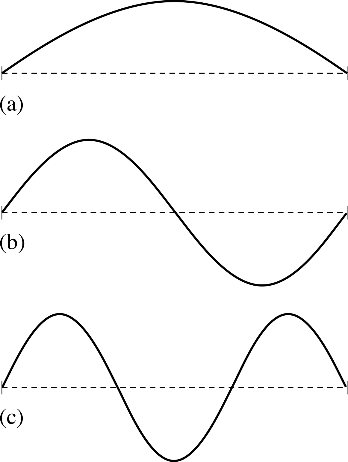
Figure 11 The three figures represent (a) the fundamental (no nodes except at the end of the string), (b) the first harmonic (one node in the middle), and (c) the second harmonic (two nodes) of standing waves on a string.
For n = 1, the value of the wavelength is the largest, while the frequency is the smallest. This smallest frequency is called the fundamental, while the higher frequencies are called harmonics. We can also characterize each allowed frequency by the number of nodes between the ends, ignoring those at each end. If we use the index n to characterize the frequency as above, then there will be (n − 1) nodes associated with the nth allowed frequency. So the fundamental exhibits zero nodes, while the first harmonic (n = 2) exhibits 1 node, and so on. Note that the nth frequency represents the (n − 1)th harmonic.
The fundamental and first two harmonics of a string are shown in Figure 11. When a string is set into motion, or excited, the only frequencies which will be of substantial intensity or duration will be the allowed frequencies described above. This means that all the frequencies present will bear a simple relationship to each other. This relationship of all the frequencies is generally pleasant to the ear, and is responsible for the musicality of stringed instruments.
Note that the fundamental frequency depends on the length of the string, the linear mass density, and the tension. The length and the linear mass density are normally fixed by the construction of a musical instrument, but the tension can be adjusted, and this is precisely how a stringed musical instrument is tuned to produce the right notes.
Question T13
The E string on a violin has a length of 0.32 m, a linear mass density of 0.38 g m−1, and is under a tension of 68 N. What are the wavelength and frequency of the fundamental and first harmonic?
Answer T13
The wavelengths and frequencies are given by:
$\lambda_1 = 2l = \rm 2\times0.32\,m = 0.64\,m$
$\lambda_2 = \dfrac{\lambda+1}{2} = \rm 0.32\,m$
$f_1 = \dfrac{1}{2l}\sqrt{\dfrac{F_{\rm T}}{\mu}} = \rm \dfrac{1}{2\times0.32\,m}\times\sqrt{\dfrac{68\,N}{0.38\,g\,m^{-1}}} = 1.56\,m^{-1}\times\sqrt{\dfrac{68\,kg\,m\,s^{-2}}{0.38\,g\,m^{-1}}}$
$\rm \phantom{f_1} = 1.56\,m^{-1}\sqrt{1.79\times10^5\,m^2\,s^{-2}} = 1.56\,m^-1\times423\,m\,s^{-1} = 660\,Hz$
f2 = 2f1 = 1300 Hz (to two significant figures)
4.5 Summary of Section 4
In this section, we have seen how the fundamental principle of superposition leads to interference effects and, when boundary conditions are imposed, to the general idea of standing or stationary waves. These are no longer travelling waves, even though their profile does change with time. Standing waves may be characterized as stationary sinusoidal waves with fixed nodes and antinodes. The presence of the fixed nodes in a standing wave leads to a unique relationship between the length of a string with fixed ends and the allowed frequencies and wavelengths that can be sustained by that string. This allows for the production of uniquely related fundamentals and harmonics, and is ultimately responsible for the musicality of stringed instruments such as the guitar and piano.
5 Waves in two or three dimensions
5.1 The wave vector
In the case of the simple one–dimensional motion we have considered so far, the direction of propagation was limited to ±x. In the case of two–dimensional waves, such as the surface waves on the ocean, or three–dimensional waves, such as the electromagnetic waves used to represent light, more information is needed to characterize the direction of propagation. In these cases this information is usually provided in the form of a wave vector k, (more properly called the angular wave vector) i which lies along the direction of propagation and has magnitude 2π/λ, where λ is the relevant wavelength.
As an example, let us consider some surface waves propagating in a horizontal (x, y) plane. These are transverse waves composed of disturbances in the (vertical) z–direction. The position of any point in the (x, y) plane can be specified by a two–dimensional vector r = (x, y), and the direction in which the waves are propagating at any point can be specified by a wave vector k = (kx, ky). For the sake of simplicity we will assume that the waves are travelling in the same direction at all points, so they are more like ocean waves in an area of open sea than the waves that spread out from a stone thrown into a pond. Under this assumption the value of k will be the same at all points, and if we look down on the (x, y) plane from above the wave crests will be seen as straight lines, at right angles to k, that are separated by one wavelength λ.
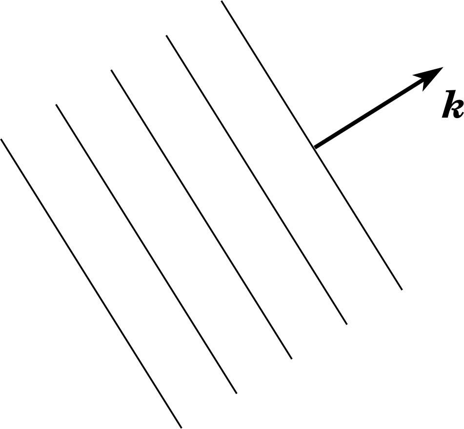
Figure 12 Parallel wave crests (more properly plane wavefronts) in a two–dimensional medium. The wave vector k is perpendicular to the wavefront, pointing in the direction of propagation, with magnitude k = 2π/λ.
Bearing in mind that the magnitude of k is $k = \sqrt{\smash[b]{k_x^2 + k_y^2}} = 2\pi\lambda$, we may if we wish say that the wave crests are separated by a distance 2π/k, and thus avoid mentioning λ altogether. This arrangement is indicated in Figure 12. If the waves are sinusoidal, the two–dimensional generalization of the one–dimensional sinusoids we discussed earlier, we can represent them mathematically by the function
z = A sin(k ⋅ r − ωt)(37)
where the term k ⋅ r represents the scalar product of the position vector r and the wave vector k. In the two–dimensional case we are considering, the value of this scalar product at a point with position coordinates (x, y) will be
k ⋅ r = kxx + kyy(38) i
It should be apparent that Equation 37 is a generalization of Equation 5,
y = A sin(kx − ωt)(Eqn 5)
since in the one–dimensional case kx = k and hence k ⋅ r = kx in that case.
Thanks to the power of vector notation, it should also be fairly obvious how we describe three–dimensional waves. In that case the wave vector will have three components so k = (kx, ky, kz), its magnitude will be
$k = \lvert\,{\boldsymbol k}\,\rvert = \sqrt{\smash[b]{k_x^2 + k_y^2 + k_z^2}} = \dfrac{2\pi}{\lambda}$
and sinusoidal waves of amplitude A involving some kind of (scalar) disturbance i Ψ can be represented by
Ψ (r, t) = A sin(k ⋅ r − ωt)
wherek ⋅ r = kx x + ky y + kz z
The waves described by Equation 37 and its three–dimensional extension are certainly not the most general kinds of two– and three–dimensional waves, but they do represent an important class of waves that you are certain to meet again in your subsequent studies. Technically they are known as plane waves since at any given time (in the three–dimensional case) all the points on any plane perpendicular to k will correspond to the same value of the phase (k ⋅ r − ωt). i
In the two–dimensional case the ‘planes’ of constant phase will just be lines and the wave crests we spoke of in Figure 12 are examples of such lines. Indeed, if we wanted to be more general we could say that the lines drawn at right angles to k in Figure 12 represent points of equal phase, irrespective of its value. Surfaces (or lines) of equal phase are generally referred to as wavefronts. It is a characteristic property of plane waves that their wavefronts are parallel planes in three dimensions and parallel straight lines in two dimensions.
Question T14
A wave–making machine causes plane waves to travel across the surface of a rectangular swimming pool. The waves have an amplitude of 30 cm, a speed of 90 cm s−1, and are produced at a frequency of 0.30 Hz. If the waves propagate at an angle of 30° to the long sides of the pool, write down a mathematical description of the waves assuming that one of the long sides of the pool is chosen to represent the x–axis.
Answer T14
The waves will be of the form
z (r, t) = A sin(k ⋅ r − ωt)
with A = 0.30 m and ω = 2πf = 0.60 π s−1 = 1.88 s−1.
k must have magnitude | k | = k = ω/υ = (1.88/0.90) m−1 = 2.09 m−1, and must be directed at 30° to the x–axis.
In terms of its components kx and ky, it is given by:
kx = k cos 30° = 1.81 m−1 and ky = ksin 30° = 1.04 m−1
Thus,z (r, t) = (0.30 m) sin[(1.81 m−1)x + (1.04 m−1)y − (1.88 s−1)t]
It should be noted that this is not the only possible correct answer to the question. For instance, you would be perfectly justified in adding an arbitrary phase constant ϕ to the phase since this would simply alter the value of the phase at x = y = 0 and t = 0, and that was not specified in the question.
5.2 Waves on a membrane
The hard (and somewhat idealized) maths is now behind us. We will conclude our discussion of waves by considering the qualitative reality of waves in two familiar contexts. First, waves on a two–dimensional elastic membrane, such as a drum membrane. i Then, in the next subsection, waves in a real (three-dimensional) ocean. In this case the waves are two–dimensional in extent, so that we are dealing with transverse motions involving two dimensions, with the propagation direction in a third.
On an elastic membrane, the boundaries are usually sufficiently close that they cannot be neglected, so we will consider finite membranes with enclosing boundaries. The drum is one of the simplest examples of this kind. In this case, the most important waves are the standing waves since they are the ones that persist and account for much of the sound that the drum produces. In one respect, the properties of standing waves on a two–dimensional membrane are similar to those of standing waves on a string with fixed ends, in that there are nodal and antinodal positions, but the description of these is more complicated. Whereas in one–dimensional systems, the nodes and antinodes are isolated points, in the case of two–dimensional standing waves, the nodes will generally be lines on the surface.
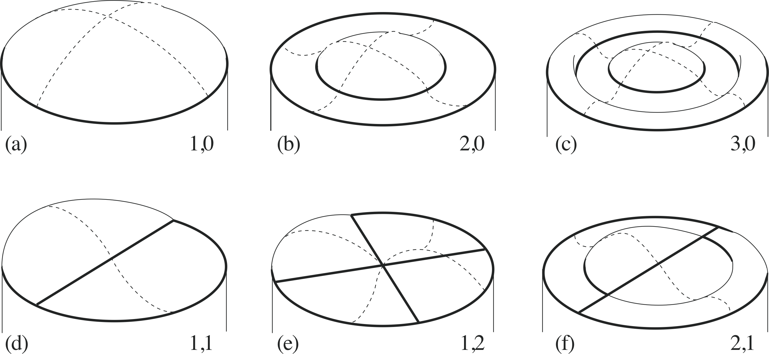
Figure 13 Six of the possible standing waves on a drum membrane. The continuous lines shown – including that around the circumference – are the nodal positions. Just as in the one–dimensional string, displacements on the opposite side of these nodes are in opposite directions.
As in the one–dimensional example, the standing waves are again determined by the boundary conditions, which in this case require that the edge of the membrane should be a nodal line. Figure 13 shows typical standing wave profiles on the surface of a drumhead.
You can see from Figure 13 that the characteristic nodal lines consist of two types, those lying along diameters of the circular membrane and those forming circles of fixed radius.
In the case of the finite one–dimensional string, we could characterize the allowed standing waves by the number of nodal points that occurred, but in the case of the drum we need to characterize both the number of nodal diameters, and the number of nodal circles in each standing wave. In general, these two–dimensional standing waves are not harmonics of the fundamental frequency, and no simple numerical relationship will exist between their frequencies and the fundamental frequency. This is probably the reason for the perceived lack of musicality of a drum.
5.3 Waves on water
We return finally to the case of water waves which is actually one of the most complex examples of mechanical waves, because of the physical nature of the system. Surface waves on water cannot be purely transverse because the water is essentially incompressible on the length scales of the surface waves with which we are familiar. This means that if we try to produce a displacement that is perpendicular to the surface of the water, other water must either enter or leave the positions vertically below the displaced surface water. (Waves that are purely longitudinal in nature depend on the compressibility of water, and these are actually what we normally call sound waves.) So although we talk about transverse waves in water, the actual motion must be a complex mixture of transverse and longitudinal movements.
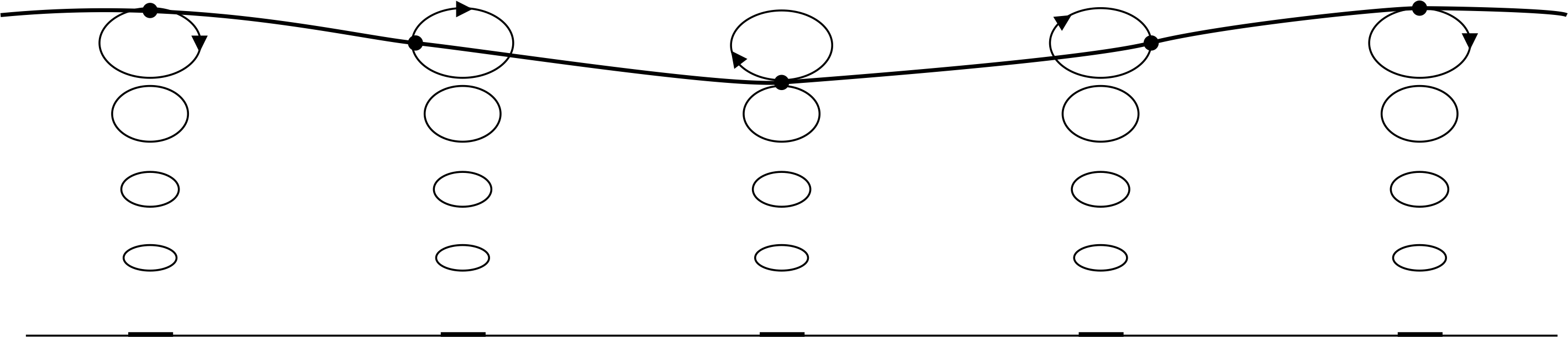
Figure 14 The motion of individual water particles involved in a transverse shallow water wave. The wave illustrated is propagating to the right.
Figure 14 indicates the nature of this motion. The motion of the surface of the water is approximately sinusoidal, although the actual motion of individual particles is more complex. Clearly, the general kinematic description of transverse waves in water is quite complicated. Each particle of water undergoes an ellipsoidal motion, moving in the direction of propagation of the wave when it is at the crest, and in the opposite direction when it is in the trough.
6 Closing items
6.1 Module summary
- 1
-
Travelling waves are disturbances that move from place to place, if they involve a medium at all they do not generally involve bulk motion of the material of that medium. In a transverse wave the disturbances that constitute the wave are at right angles to the direction of propagation.
- 2
-
A transverse wave that propagates in the +x–direction with constant phase speed υ and without changing its shape may be described by a function of two variables of the form
y = f (x ± υt)(Eqn 1)
A more specialized but common example of this is the sinusoidal wave
y = A sin(kx ± ωt)(Eqn 5)
expressed using the angular wavenumber k and the angular frequency ω. This can be rewritten in equivalent forms using other parameters such as the (linear) frequency f, the period T, the wavelength λ, and the wavenumber σ.
These quantities are related in the following ways:
$\omega = \dfrac{2\pi}{T}\quad f = \dfrac1T\quad k = \dfrac{2\pi}\lambda\quad\sigma = \dfrac1\lambda$
$\upsilon = \lambda f = \dfrac{\omega}{k} = \dfrac{\lambda}{T}$
- 3
-
Newton’s laws applied to the transverse motion of a string produce the equation:
$\dfrac{\partial^2y}{\partial x^2} = \dfrac{\mu}{F_{\rm T}}\dfrac{\partial y}{\partial t^2}$(Eqn 15)
where μ is the mass per unit length of the string and FT is the magnitude of the tension in the string.
Comparing this with the general one–dimensional wave equation,
$\dfrac{\partial^2{\it\Psi}}{\partial x^2} = \dfrac{1}{\upsilon^2}\dfrac{\partial{\it\Psi}}{\partial t^2}$(Eqn 25)
shows that the phase speed of waves on a string is $\upsilon = \sqrt{F_{\rm T}/\mu}$.
- 4
-
The linear energy density of a string which carries transverse sinusoidal displacement waves is also a wave, with the same phase speed but half the wavelength and double the frequency of the displacement wave:
$D_E(x,t) = \dfrac{\mu\omega^2A^2}{2}\left[1 + \cos(2kx - 2\omega t)\right]$
The rate at which energy is transferred by such waves is proportional to the square of the amplitude and the square of the angular frequency.
- 5
-
The superposition principle allows us to construct new solutions of the (linear) wave equation out of linear combinations of known solutions. This leads to the phenomenon of interference, and also accounts for the group velocity observed when wave groups (a superposition of waves with closely similar frequencies) travel through a medium which gives rise to dispersion.
- 6
-
The boundary conditions describing wave behaviour at the ends of strings, together with the superposition principle, lead to standing waves on strings, which have nodes and antinodes with spacings determined by the wavelength of the standing waves. On finite strings with fixed ends, these lead to conditions on the possible values of wavelength and frequency for waves which can be sustained by the string. This in turn leads to the existence of a regularly spaced sequence of sustainable frequencies, the fundamental and its harmonics, and to the basic musicality of stringed musical instruments.
- 7
-
In the case of waves in more than one dimension, the concept of the angular wavenumber must be generalized to the (angular) wave vector, which allows for a compact expression of a three–dimensional wave:
Ψ (r, t) = A sin(k ⋅ r − ωt)
wherek ⋅ r = kx x + ky y + kz z and $k = \lvert\,{\boldsymbol k}\,\rvert = \sqrt{\smash[b]{k_x^2 + k_y^2 + k_z^2}} = \dfrac{2\pi}{\lambda}$
- 8
-
A generalization of standing waves on strings to two dimensions has its most familiar expression in the standing waves on a bounded membrane such as a drum. The standing waves are two-dimensional, and there is no longer a regular spacing for the allowed sequence of frequencies.
6.2 Achievements
Having completed this module, you should be able to:
- A1
-
Define the terms that are emboldened and flagged in the margins of the module.
- A2
-
Describe the mathematical form of a general travelling wave pulse.
- A3
-
Define and use the terms (angular) frequency, period, wavelength, (angular) wavenumber displacement and amplitude as applied to periodic travelling waves.
- A4
-
Relate the frequency and wavelength of a sinusoidal wave to its phase speed.
- A5
-
Describe the relationship between the force law on a string and transverse waves on a string.
- A6
-
Understand and be able to use the relationship between υ, FT and μ for transverse waves on a string.
- A7
-
Describe the characteristics of the energy density in waves and be able to calculate energy densities for transverse sinusoidal waves on strings.
- A8
-
Write down the generalized one–dimensional wave equation, and explain the nature of the partial derivatives that it contains. (You should be able to determine partial derivatives in a few simple cases, but a general mastery of partial differentiation is not expected.)
- A9
-
State the principle of superposition and use it in various simple cases, including those involving interference and wave group speed.
- A10
-
Explain the reflection of transverse waves at a rigid boundary, and describe reflection at a free boundary.
- A11
-
Describe the production of standing waves on a string, and interpret mathematical representations of simple standing waves.
- A12
-
Explain the significance of boundary conditions for the standing waves on a string with fixed ends, and derive the relationships between nodal and antinodal positions in such cases.
- A13
-
Describe the relationship of standing waves to stringed musical instruments.
- A14
-
Describe the behaviour of transverse waves in two and three dimensions and be able to recognize, use and interpret mathematical representations of sinusoidal plane waves in two and three dimensions.
Study comment You may now wish to take the following Exit test for this module which tests these Achievements. If you prefer to study the module further before taking this test then return to the topModule contents to review some of the topics.
6.3 Exit test
Study comment Having completed this module, you should be able to answer the following questions each of which tests one or more of the Achievements.
Question E1 (A3)
A person observes water waves moving past and finds that the time taken for five crests to pass by is 8.0 s (i.e. four complete waves), with the distance between successive crests being 4.0 m. What is the speed of these water waves? What is the angular frequency?
Answer E1
The timing is for the passage of five crests, so that the interval represents four periods. The distance between crests is just the wavelength, so we calculate:
$T = \rm \dfrac{8.0\,s}{4} = 2.0\,s$
hence$\upsilon = \dfrac{\lambda}{T} = \rm \dfrac{4\,m}{2.0\,s} = 2.0\,m\,s^{-1}$
and$\omega = \dfrac{2\pi}{T} = \pi\,{\rm s^{-1}} = 3.1\,{\rm s^{-1}}$
(Reread Subsections 2.2 and 2.3 if you had difficulty with this question.)
Question E2 (A3 and A4)
A sinusoidal wave has an amplitude of 3 cm, a period of 5 s and a phase speed of 15 cm s−1. Give the mathematical function y (x, t) that describes this wave. Assume that at t = 0 and x = 0, the displacement is 3 cm.
Answer E2
An appropriate form for the function is y = A cos k (x ± υt), which gives a maximum at x = 0 and t = 0. We just need k, which we can find easily from:
$k = \dfrac{\omega}{\upsilon} = \dfrac{2\pi}{\upsilon T} = \rm \dfrac{2\pi}{15\,cm^{-1}\times5\,s} = \dfrac{2\pi}{75\,cm} = 8.4\times10^{-2}\,cm^{-1}$
hencey = 3 cos[(8.4 × 10⁻² cm−1)(x − (15 cm s−1)t)]
where y and x are measured in cm, and t in s.
(Reread Subsection 2.3 if you had difficulty with this question.)
Question E3 (A6)
A wire with a mass of 0.1 kg is tautly strung between two walls 10.0 m apart. If the wire is under a tension of 100 N, how long will it take a transverse pulse to travel from one wall to the other?
Answer E3
The mass is 0.1 kg and the length is 10.0 m, so the linear mass density is 0.01 kg m−1. The time of travel ∆t will be given by l/υ, so we need υ:
$\upsilon = \sqrt{\dfrac{F_{\rm T}}{\mu}} = \rm \sqrt{\dfrac{100\,kg\,m\,s^{-2}}{0.01\,kg\,m^{-1}}} = \sqrt{10^4\,m^2\,s^{-2}} = 100\,m\,s^{-1}$
Then ∆t = 10.0 m/100 m s−1 = 0.1 s.
(Reread Subsection 2.6 if you had difficulty with this question.)
Question E4 (A4 and A9)
Two sinusoidal waves with the same wavelength and amplitude are travelling in opposite directions on a string, with the same phase speed of 20 cm s−1. If the time interval between moments when the string is perfectly flat is 0.5 s, what is the wavelength? Describe the appearance of the string 0.25 s after it is flat.
Answer E4
The string will be flat when the maxima of one wave coincide with the minima of the second. The next time this will occur is when the waves have moved one wavelength with respect to each other. Since the relative speed of the two waves is twice the phase speed, we have the wavelength given by:
λ = 2υ∆t = 2 × 20 cm s−1 × 0.5 s = 20 cm.
After 0.25 s, the waves have travelled one–half wavelength with respect to each other, which means that the maxima (and minima) of the two waves will coincide now. Thus we will instantaneously observe a sine wave with twice the amplitude of the individual waves.
(Reread Section 3 if you had difficulty with this question.)
Question E5 (A3 and A7)
A travelling sinusoidal wave is described by the equation
y = (5 cm) cos[(10 m−1)x − (4 s−1)t]
where y and x are measured in centimetres and t is measured in seconds. If the wave is on a wire with a linear mass density of 3 × 10⁻³ kg m−1, what are the amplitude and wavelength of the corresponding linear energy density wave?
Answer E5
If the displacement wave is given by y = A cos(kx − ω1t), the linear energy density wave can generally be written as
$D_E(x,t) = \dfrac{\mu\omega^2A^2}{2}\left[1 + \cos(2kx - 2\omega t)\right]$
so in this case
$D_E(x, t) = \frac12 (3\times10^{-3}\,{\rm kg\,m^{-1}})(4\,{\rm s^{-1}})^2(5\times10^{-2}\,{\rm m})^2\times\left\{1 + \cos\left[(20\,{\rm m^{-1}})x - (8\,{\rm s^{-1}})t)\right]\right\}$
$\phantom{D_E(x, t) }= 6\times10^{-5}\,{\rm J\,m^{-1}}\left\{1 + \cos\left[(20\,{\rm m^{-1}})x - (8\,{\rm s^{-1}})t)\right]\right\}$
so the amplitude is 0.06 J mm−1 and the wavelength is (2π/20) m = 0.31 m.
(Reread Subsection 2.7 if you had difficulty with this question.)
Question E6 (A9 and A11)
A nylon guitar string has a linear mass density of 7.0 g m−1, a length of 80 cm, and is under a tension of 200 N. Standing waves are excited on the string and there are two nodes present between the ends of the string. Calculate the phase speed, wavelength and frequency of the waves that have been generated on the string.
Answer E6
There are two nodes in the standing wave pattern; since the number of nodes (apart from the clamped ends) equals n = 2, this means that the second harmonic is excited. The phase speed is given by:
$\upsilon = \rm \sqrt{\dfrac{200\,kg\,m\,s^{-2}}{7\times10^{-3}\,kg\,m^{-1}}} = \sqrt{2.86\times10^4\,m^2\,s^{-2}} = 169\,m\,s^{-1}$
The wavelength is:
λ = 2l/n = 2 × 80 × 10−2 m/3 = 0.53 m
The frequency is given by:
f = υ/λ = 169 m s−1/0.53 m = 317 Hz
(Reread Subsections 4.3 and 4.4 if you had difficulty with this question.)
Question E7 (A13)
Middle C on a piano has a frequency of 261.6 Hz. If a person can hear sounds up to a maximum frequency of 20 kHz, what is the highest audible harmonic of middle C?
Answer E7
The fundamental frequency is 261.6 Hz, and harmonic frequencies are given by n × 261.6 Hz. We thus want the largest integer such that this product is less than 20 kHz. Therefore n ≤ 200 00/261.6 = 76.5, so that the value of n is 76, which represents the 75th harmonic.
(Reread Subsections 4.3 and 4.4 if you had difficulty with this question.)
Study comment This is the final Exit test question. When you have completed the Exit test go back and try the Subsection 1.2Fast track questions if you have not already done so.
If you have completed both the Fast track questions and the Exit test, then you have finished the module and may leave it here.
Study comment Having seen the Fast track questions you may feel that it would be wiser to follow the normal route through the module and to proceed directly to the following Ready to study? Subsection.
Alternatively, you may still be sufficiently comfortable with the material covered by the module to proceed directly to the Section 6Closing items.