PHYS 5.4: AC circuits and electrical oscillations |
PPLATO @ | |||||
PPLATO / FLAP (Flexible Learning Approach To Physics) |
||||||
|
1 Opening items
1.1 Module introduction
Perhaps before reading this module you should do a small electrical audit. Spend a minute or two wandering around your home looking at the electrical appliances which you find there. Most of them will have a small plate or sticker attached which tells you something about their electrical specifications. My toaster, which is quite a simple model, just says 240 V 1000 W 50 Hz. Whilst the back of my microwave – which incidentally was made in France – bears the more complicated legend
240 V ~ 50 Hz
fréq.: 2450 MHz
MW 1500 W/6,5 A
A good deal of this information concerns the sort of power supply that the appliance requires. In both the cases quoted the appliance requires a supply of alternating current (a.c.), with a root-mean-square voltage of 240 volts and a frequency of 50 hertz. Alternating currents are the central theme of this module. It seems clear that we must know something about them if we are to understand even the most basic information written on electrical appliances. (From 1995 the UK electricity supply was 230 volts.)
Section 2 begins by showing a mathematical way of describing alternating currents, and investigating their behaviour in various electronic circuit components. This involves building mathematical models of physical situations, a process that some students find daunting. To avoid confusion everything has been made as explicit as possible, so you may find some of the steps spelled out in rather a lot of detail. Other topics covered in Section 2 include impedance (the a.c. equivalent of resistance), and the construction of simple filter circuits that can be used to block signals in certain frequency ranges. Phasor methods are introduced and used in this discussion to determine the impedances (and other properties) of a variety of simple circuits.
Section 3 uses the results and concepts introduced in Section 2 to study the behaviour of charge, current and voltage in a variety of simple circuits. The circuits studied can exhibit various kinds of short–lived transient behaviour and, in some cases, sustained oscillations in which charges and currents flow back and forth repeatedly between different circuit components. In the most complicated cases this can even result in resonance when an alternating electrical supply excites an unusually large response from an appropriately designed circuit. This discussion of transients and oscillations also introduces the idea of a differential equation and some of the general principles that surround the use of such equations in particular physical contexts. However, no attempt is made to teach the mathematical techniques that are required to solve such equations in general.
Although most people have some understanding of direct current, it is alternating current which – in many ways – has the greatest bearing upon our lives. That is one of the reasons why this module is important since it deals with an aspect of electricity which impinges directly upon our everyday lives.
Study comment Having read the introduction you may feel that you are already familiar with the material covered by this module and that you do not need to study it. If so, try the following Fast track questions. If not, proceed directly to the Subsection 1.3Ready to study? Subsection.
1.2 Fast track questions
Study comment Can you answer the following Fast track questions? If you answer the questions successfully you need only glance through the module before looking at the Subsection 5.1Module summary and the Subsection 5.2Achievements. If you are sure that you can meet each of these achievements, try the Subsection 5.3Exit test. If you have difficulty with only one or two of the questions you should follow the guidance given in the answers and read the relevant parts of the module. However, if you have difficulty with more than two of the Exit questions you are strongly advised to study the whole module.
Question F1
An inductor L of value 0.50 H, a resistor R of value 10 Ω and a capacitance C of value 5.07 μF are connected in series (an LCR circuit) to an alternating supply of frequency 100 Hz. What is the total impedance due to the three components? If the rms value of the supply voltage is 120 V calculate the peak value of the resulting current. What is the phase relationship between the current and the voltage?
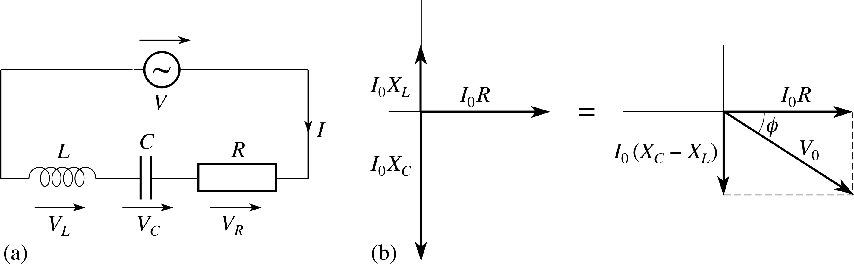
Figure 13 A series LCR a.c. circuit with the relevant phasor diagram showing how the individual voltages are combined. (In this case XC > XL).
Answer F1
The impedance of the series LCR circuit (see Figure 13) is given by
$Z = \sqrt{\smash[b]{R^2 + (X_L - X_C)^2}}$
$\vphantom{Z }= \sqrt{R^2 + \left(\omega L - \dfrac{1}{\omega C}\right)^2}$
where ω = 2π × 100 Hz.
So,
$Z = \sqrt{(10)^2 + \left(2\pi\times100\times0.5-\dfrac{1\times10^6}{2\pi\times100\times5.07}\right)^2}\,\Omega = 10\,\Omega$
So, XC ≈ XL.
The rms voltage is related to the peak voltage by $V_{\rm rms}= V_0/\sqrt{2\os}$. So in this case V0 = 169.7 V.
But the peak current is given by I0 = V0/Z, so I0 = 169.7 V/10 Ω = 17.0 A
Because the total reactance XL − XC is negligible in this case the current in the circuit will be in phase with the supply voltage.
Question F2
Starting from an appropriate condition concerning the total voltage drop around a circuit, show that the current I (t) in a series LCR circuit that contains an external voltage supply V0 sin(Ωt) must satisfy an equation of the form:
$L\dfrac{d^2I}{dt^2} + R\dfrac{dI}{dt} + \dfrac{I(t)}{C} = V_0{\it\Omega}\cos({\it\Omega}t)$
Describe the eventual behaviour of the general solution to this equation, after any transients have decayed.
Figure 13 A series LCR a.c. circuit with the relevant phasor diagram showing how the individual voltages are combined. (In this case XC > XL).
Answer F2
Following the sign conventions indicated in Figure 13, the appropriate condition on the voltage drops is
VC(t) + VR(t) + VL(t) = V0 sin(ωt)
But$V_C(t) = \dfrac{q(t)}{C}$;
$V_R(t) = I(t)R = R\dfrac{dq}{dt}$
and$V_L(t) = L\dfrac{dI}{dt} = L\dfrac{d^2q}{dt^2}$
where q (t) represents the charge on the right–hand plate of the capacitor.
So$L\dfrac{d^2q}{dt^2} + R\dfrac{dq}{dt} + \dfrac{q(t)}{C} = V_0\sin({\it\Omega}t)$
Taking the derivative of both sides with respect to t, and using the rules
$\dfrac{d}{dt}[kf(t)] = k\dfrac{df}{dt}\quad\text{and}\quad\dfrac{d}{dt}[\sin(kt)] = k\cos(kt)$
where k is a constant and f (t) a function of t, we find that
$L\dfrac{d^2I}{dt^2} + R\dfrac{dI}{dt} + \dfrac1C \dfrac{q}{dt} = V_0{\it\Omega}\cos({\it\Omega}t)$
but,dq/dt = I (t)
so$L\dfrac{d^2I}{dt^2} + R\dfrac{dI}{dt} + \dfrac{I(t)}{C} = V_0{\it\Omega}\cos({\it\Omega}t)$
After transients have decayed the remaining oscillation will be excited by the driving voltage and will be of the form
I (t) = A sin(Ωt + ϕ), where A and ϕ are constants whose values depend on Ω.
1.3 Ready to study?
Study comment In order to study this module you will need to be familiar with the following terms: amplitude, capacitance, charge, current, frequency, Kirchhoff’s laws, parallel circuit, period, power, Ohm’s law, oscillation, radians, resistance, series_connectionseries circuit, simple harmonic motion, vector (and vector addition) and voltage. Mathematically, you should be familiar with the trigonometric functions sin (θ) and cos (θ) (including their graphs) and the use of the arctaninverse trigonometric function arctan (x) to solve equations of the form tan(θ) = x. You will also need to know Pythagoras’s theorem and to be familiar with trigonometric identities, including the following results:
$\sin^2(\theta)+\cos^2(\theta) = 1,\;\sin(\theta) = \cos\left(\theta - \dfrac{\pi}{2}\right),\;\cos(\theta) = \left(\theta + \dfrac{\pi}{2}\right) \;\text{and}\;\cos(\theta) = -\sin\left(\theta - \dfrac{\pi}{2}\right)$ i
You do not need to be fully conversant with differentiation in order to study this module, but you should be familiar with the calculuscalculus notation dx/dt used to represent the rate of change of x with respect to t. If you are uncertain about any of these definitions then you can review them now by reference to the Glossary, which will also indicate where in FLAP they are developed. In addition, you will need to be familiar with SI units. The following Ready to study questions will allow you to establish whether you need to review some of the topics before embarking on this module.
Question R1
A 50 Ω resistor is connected to a 120 V d.c. supply. Calculate the current flowing in this resistor and hence the energy dissipated as heat in 5 min.
Answer R1
Using Ohm’s law V = IR, we find that the current flowing is
I = 120 V/50 Ω = 2.40 A
Power dissipation is given by
P = VI = I 2R
The total energy dissipated in time t is therefore
E = Pt = I 2Rt
i.e.E = (2.40 A)2 × 50 Ω × (5 × 60 s) = 86.4 kJ
Consult Ohm’s law and power dissipation in the Glossary for further information.
Question R2
A 100 μF capacitor is connected to a 6 V d.c. supply until it is fully charged. Calculate the maximum charge on the capacitor. If this capacitor is then discharged through a 10 Ω resistor, calculate the maximum current which will flow.
Answer R2
The maximum charge on the capacitor is given by q = VC. Hence
q = (6 V × 100 μF) = 600 μC
The maximum current flow is that which will flow initially. It is given by I = V/R = (6 V/10 Ω) = 0.6 A. The current, or rate of flow of charge, decreases thereafter.
Consult charge and capacitor in the Glossary for further information.
Question R3
A resistor and a capacitor are connected in series_connectionseries to a d.c. supply. Draw a diagram representing this electrical circuit. The two components are now re–connected in parallel with the same d.c. supply. Draw a diagram representing this new circuit.
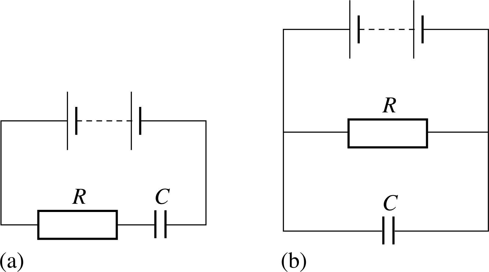
Figure 26 See Answer R3.
Answer R3
The series and parallel circuit diagrams are shown in Figure 26a and b, respectively.
Consult series_connectionseries and parallel_connectionparallel circuit diagrams in the Glossary for further information.
Question R4
The displacement of a sinusoidal oscillation is described by the expression y = A sin(2πft), where A = 10 cm and f = 2 Hz. Calculate the displacement y when t = 0.25, 0.30 and 0.70 s, respectively. What is the period of this oscillation?
Answer R4
Since y = A sin(2πft), and given that the amplitude A is 10 cm and frequency f is 2 Hz, we can calculate the displacement at various times as follows. (Don’t forget to use the radian mode on your calculator.)
When t = 0.25 s, y = 10 cm × sin(2π × 2 s−1 × 0.25 s) = 10 cm × sin π = 0 cm
Similarly, when t = 0.30 s, y = −5.88 cm, and when t = 0.70 s, y = +5.88 cm.
The period is related to the frequency by T = 1/f. Hence T = 1/(2 s−1) = 0.50 s.
Consult the relevant terms in the Glossary for further information.
2 AC circuits
2.1 Describing alternating currents and voltages
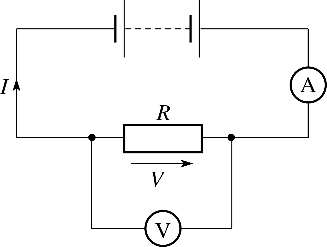
Figure 1 A simple d.c. circuit showing the measurement of potential difference and current using a voltmeter and ammeter, respectively. The arrow associated with the (conventional) current I indicates the direction in which positive charges would flow. The arrow associated with the voltage drop across the resistor points from low to high voltage and opposes the current direction. Negative values for I or V indicate currents and voltage drops that oppose the respective arrows.
You should already be familiar with the properties of a simple d.c. circuit of the kind shown in Figure 1. The box symbol represents a resistor, and the battery symbol represents a source of voltage (i.e. potential difference). The current I in the circuit will be such that the voltage drop V across the resistance R is equal to the voltage supplied by the battery. The voltage drop across the resistor can be measured using a voltmeter connected in parallel whilst the current flowing through the resistor can be measured using an ammeter connected in series. The resistance R can then be determined using Ohm’s law
$R = \dfrac VI$(1) i
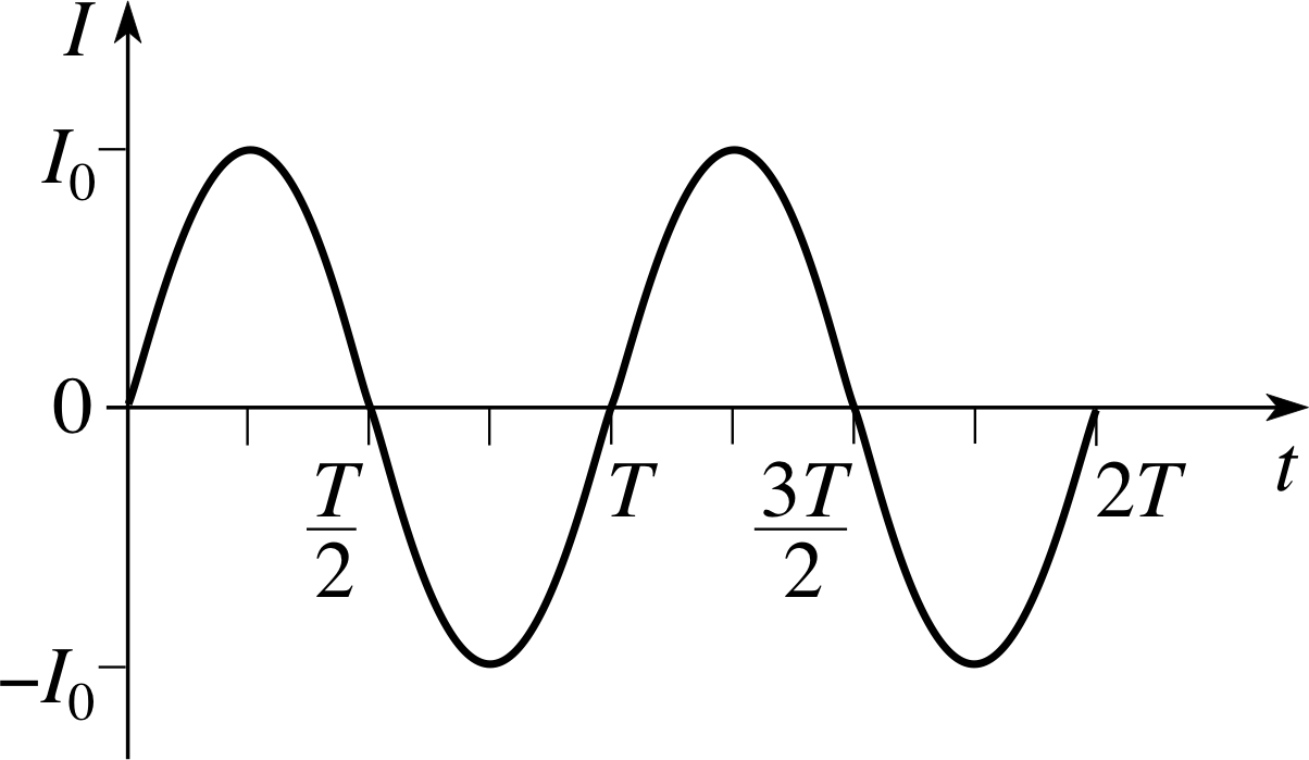
Figure 2 Two cycles of an alternating current with peak value I0 and period T. Such a current may be represented by the function
In analysing a d.c. circuit such as that of Figure 1 we generally think of the battery as a source of constant voltage, so that the current in any part of the circuit is a steady flow of electric charge in a single direction; that, after all, is the meaning of d.c. – direct current. However, not all voltage sources are constant and neither are all currents direct. For example, the mains voltage supplied by standard wall sockets in the UK varies rapidly with time, the potential difference between the ‘live’ and ‘neutral’ terminals changing not just in magnitude but even in sign 50 times a second. Not surprisingly, the currents that such varying voltages produce in circuits will also vary with time, generally altering both their magnitude and direction in response to the variations in the voltage. A current that periodically reverses its direction in this way is called an alternating current (a.c.).
The simplest kind of alternating current is represented in Figure 2. The current changes smoothly and regularly with time in a manner that may be described by a sinusoidal function (i.e. a sine or a cosine function), just like a simple harmonic oscillator. Its peak value (or amplitude) is I0, and the period over which it goes through one complete oscillatory cycle is T. In drawing Figure 2 we have chosen the time t = 0 to be a moment at which the current is zero, consequently, it is marginally easier to represent this particular current by means of a sine function rather than a cosine function so we can write
$I(t) = I_0\sin\left(\dfrac{2\pi t}{T}\right)$(2)
Note that we have chosen to represent the current by I (t) in order to emphasize that the value of I is changing with time and will generally depend on the value of t at which we choose to measure it.
Equation 2 is very similar in form to the equation used to describe the displacement of a simple harmonic oscillator from its equilibrium position. The quantity 2πt/T, is called the phase of the oscillator, and increases by 2π each time t increases by an amount T.
Since an increase of phase by 2π corresponds to a complete oscillation, the phase has many of the characteristics of an angle measured in radians and some authors prefer to treat it as an angle, in which case it may be called the phase angle.
It is possible to write the phase in Equation 2 in a couple of other ways. The frequency f of an oscillation is related to the period by f = 1/T, so it is always possible to replace 2πt/T by 2πft. More usefully we can introduce a related quantity called the angular frequency which is defined by ω = 2π/T so that the phase 2πt/T may be simply written as ωt.
In terms of frequency and angular frequency, the alternating current described by Equation 2 may therefore be written in the following equivalent ways.
$I(t) = I_0\sin(2\pi ft)$(3a)
$I(t) = I_0\sin(\omega t)$(3b)
where f = 1/T and ω = 2π/T
Frequency and angular frequency are defined in such a way that either quantity may be measured in units of s−1, thus the SI unit of each quantity is the hertz (Hz) since 1 Hz = 1 s−1.
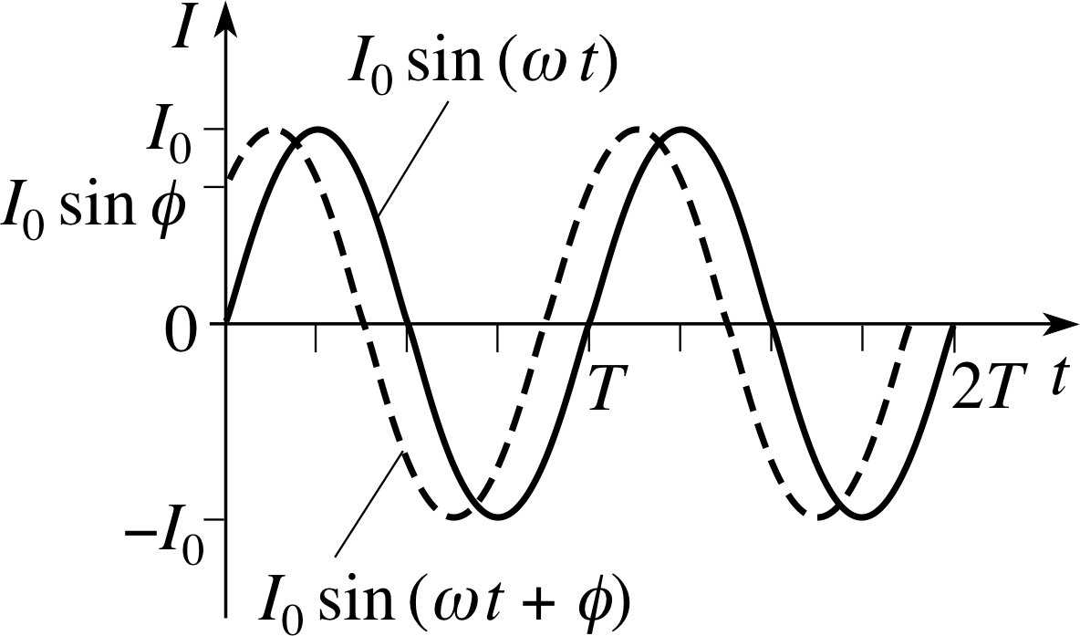
Figure 3 Sketch graph showing I1 = I0 sin(ωt) and I2 = I0 sin(ωt + ϕ), in which I2 leads I1 by a phase constant ϕ.
So far, our mathematical descriptions of alternating currents have all been limited to the case where I = 0 when t = 0. Obviously this need not be the case; it is quite possible for an alternating current to have any one of its allowed values at t = 0. Figure 3 indicates the general situation that can arise. The current I1 is of the kind we have already discussed and is described by:
I1(t) = I0 sin(ωt)(4a)
but the current I2, which has the same angular frequency and amplitude as I1, has some other value at t = 0. This more general current may be represented by the expression
I2(t) = I0 sin(ωt + ϕ)(4b)
where the constant ϕ is called the phase constant. The phase constant is the value of the phase at t = 0 and determines the current at that time since I2(0) = I0 sin ϕ.
Given any two quantities that oscillate with the same angular frequency, such as I1 and I2, it is always possible to relate the oscillations of one to those of the other by describing the way in which the phase of one is related to that of the other. In the case of I1 and I2 we can describe this phase relationship by saying that I2 phase_leadleads I1 by ϕ or that I1 phase_laglags I2 by ϕ. Note that ϕ could have many values, though it is customary to limit it to the range −π < ϕ ≤ +π since adding or subtracting an integer multiple of 2π to the phase makes no difference to the value of the current.
Figure 2 Two cycles of an alternating current with peak value I0 and period T. Such a current may be represented by the function
✦ (a) Use the trigonometric identity sin(θ) = cos θ − π to write down an expression that represents the current I shown in Figure 2 in terms of a cosine function.
(b) Use the trigonometric identity cos(θ) = sin θ + π to determine the phase relationship between cos(ωt) and sin(ωt).
✧ (a) $I(t) = I_0\sin\left(\dfrac{2\pi t}{T}\right) = I_0\cos\left(\dfrac{2\pi t}{T}-\dfrac{\pi}{2}\right) = I_0\cos\left(\omega t-\dfrac{\pi}{2}\right)$
(b) Using the given identity we see that cos(ωt) = sin(ωt + π/2), so it must be the case that the cos(ωt) leads sin(ωt) by π/2, or equivalently, that sin(ωt) lags cos(ωt) by π/2. This result will be very useful later in this module.
The phasor representation
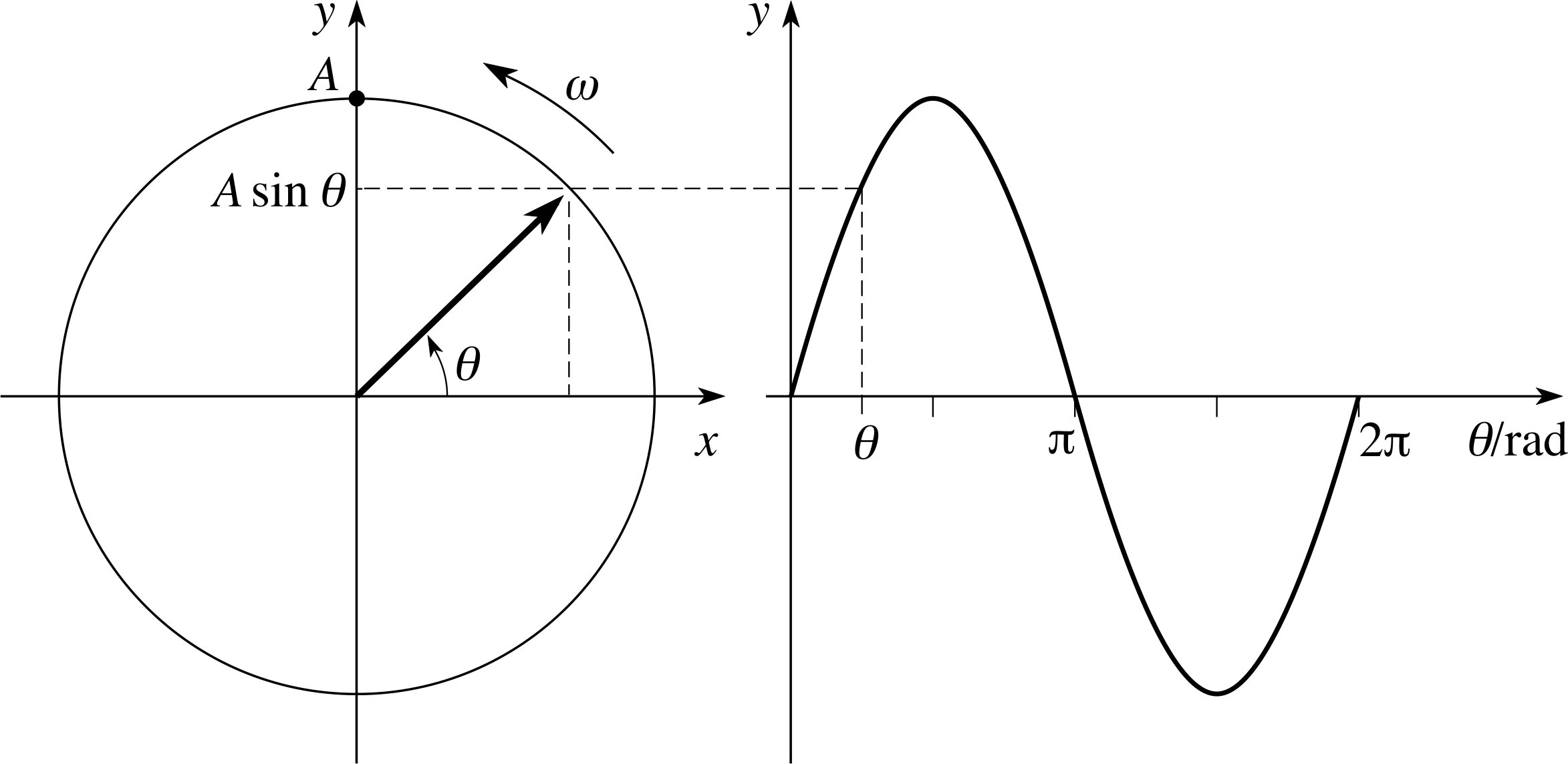
Figure 4 The projection of a phasor on to the y–axis is a sinusoidal function of the angle θ.
Another way of representing the alternating current of Figure 2 is in terms of a rotating phasor, as shown in Figure 4. A phasor is rather like the hand on a clock, though the phasors we will consider will all rotate in the anticlockwise direction. A phasor has a magnitude A and rotates at a fixed angular speed ω, so that the angle θ from the x–axis to the phasor increases with time. i The y–component of the phasor (i.e. its ‘projection’ y = A sin θ on to the y–axis) varies sinusoidally with θ, as indicated in Figure 4.
It follows that a graph showing the variation of this y–component with time will be identical to Figure 2 provided the following requirements are met:
- 1
-
The magnitude A of the phasor is equal to the amplitude (or peak value) I0 of the current.
- 2
-
At any time t, the angle θ of the phasor is equal to the phase (generally, ωt + ϕ) of the current.
Question T1
Draw a diagram showing the phasors that represent the alternating currents I1 and I2 (defined in Equations 4a and 4b) at time t = 0. In what way would your answer have changed if you had been asked to draw the phasors a quarter of a period later, at t = T/4?
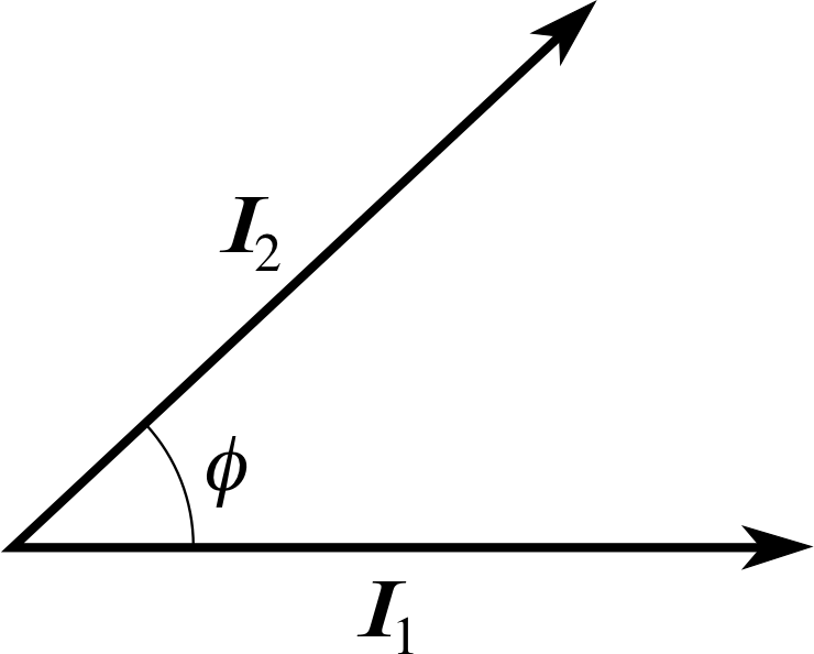
Figure 27 See Answer T1.
Answer T1
Phasors representing the alternating currents I1 and I2 at time t = 0 are shown in Figure 27. A quarter of a period later both phasors would have turned through 90° in the anticlockwise direction. Note that the phasors have been labelled by bold letters I1 and I2 to distinguish them from the currents which are represented by the vertical component of the corresponding phasor.
The fact that oscillating systems, such as alternating currents, can be represented by phasors is interesting but little more than that at present. However, later in the module you will see that the phasor representation becomes very useful when we have to work out the combined effect of several alternating currents that differ in phase and amplitude.
2.2 AC power and rms current
When dealing with direct current, the power dissipated by a current passing through a resistor may be calculated using the formula
P = I 2R(5)
Resistors can become hot as a result of this power dissipation when current passes through them.
When dealing with alternating current the situation is not so simple, since the current changes continuously. If the current at any instant is given by I = I0 sin(ωt), then the instantaneous a.c. power dissipation is given by
P = I 2R = I02R sin2(ωt)
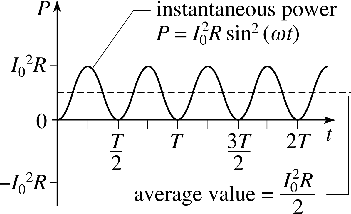
Figure 5 The instantaneous power dissipation $P = I_0^2R\sin^2(\omega t)$.
This instantaneous power is shown in Figure 5. Though it is useful to know the expression for the instantaneous power it is not really of much direct relevance when dealing with everyday a.c. devices such as light bulbs and electric heaters. The frequency of the mains supply (50 Hz in the UK) is such that the instantaneous power rises and falls 100 times every second, which is much too fast for any changes in heating effect to be seen or felt. When dealing with such everyday devices it is more useful to have an expression for the average a.c. power dissipated over a time that is much larger than the oscillation period of the current.
Over one complete period of oscillation T, the average value of an alternating current I = I0 sin(ωt) will be zero since every positive contribution to the average current will be counterbalanced by a negative contribution of equal magnitude. Nonetheless, an alternating current really does cause power dissipation in a resistor – you only have to switch on an electric fire to be sure of that. The reason for this is apparent from Equation 5: the instantaneous power is proportional to I 2, so the instantaneous power is positive whenever I is non-zero, irrespective of its sign.
Thus, the average power $\langle P\rangle$ i dissipated over one full period T will be equal to the mean of I 2 over that period. We may indicate this by using angular brackets to denote the mean and writing
$\langle P\rangle = \langle I^2R\sin^2(\omega t) = I^2R\langle\sin^2(\omega t)\rangle$ i
Now the mean square current on the right–hand side can be worked out straightforwardly using the techniques of integration developed elsewhere in FLAP, but there is a simpler method that uses the special properties of the function sin2(ωt). Since the angular brackets indicate an average over a full period of oscillation, the time at which we start timing is unimportant, so we could equally well write
$\langle P\rangle = \langle I^2R\sin^2(\omega t) = I^2R\langle\cos^2(\omega t)\rangle$ i
If we add the right–hand sides of these last two equations we find:
$2\langle P\rangle = \langle I^2R\sin^2(\omega t) + \langle I^2R\cos^2(\omega t) = I^2R\langle\sin^2(\omega t) + cos^2(\omega t)\rangle$
However sin2(ωt) + cos2(ωt) = 1, which is a constant, so its average value over a full period is the same as its instantaneous value, i.e. 1.
Thus,
$\langle\sin^2(\omega t) + cos^2(\omega t)\rangle = 1$
so$2\langle P\rangle = I_0^2R$
i.e.$\langle P\rangle = \dfrac12 I_0^2R$(6)
This amounts to saying that $\langle\sin^2(\omega t)\rangle = 1/2$, so the mean of I 2 over a full period is I02/2.
As you can see, when an alternating current of peak value I0 passes through a resistance R, the power dissipation is the same as that which would occur if a direct current of steady value I0/2 were to flow through the resistor. Because of the way it has been derived – by taking the square root of the mean of I 2 over a full period – this ‘effective average current’ is called the root_mean_square_r.m.s._currentroot–mean–square current or root_mean_square_r.m.s._currentrms current. The root-mean-square current is usually denoted Irms so we can write:
$\langle P\rangle = I_{\rm rms}^2R$(7a)
where$I_{\rm rms} = I_0/\sqrt{2\os} = 0.70171 I_0$(8a)
If we had started this investigation of the power dissipated by a resistor connected to an a.c. supply by considering an alternating voltage V = V0 sin(ωt) across the resistor rather than an alternating current through the resistor, we could have used the d.c. expression P = V 2/R to lead us to the a.c. results:
$\langle P\rangle = \dfrac{V_{\rm rms}^2}{R}$(7b)
where$V_{\rm rms} = V_0/\sqrt{2\os} = 0.70171 V_0$(8b)
In this case Vrms is the root_mean_square_r.m.s._voltageroot–mean–square voltage. Finally, note that by multiplying together the right–hand sides of Equations 7a and 7b, and then taking the square root, it can be seen that the average power dissipated by the resistor is also given by:
$\langle P\rangle = V_{\rm rms}I_{\rm rms}$(7c) i
Question T2
A 10 Ω resistor is supplied using a 6 V d.c. supply. Calculate the following quantities:
(a) The current flowing through the resistor.
(b) The energy dissipated every second in the resistor.
(c) The rms current and rms voltage which would produce identical energy dissipation with the resistor connected to an alternating supply.
(d) The corresponding peak values of alternating voltage and current.
Answer T2
(a) I = V/R = 6 V/10 Ω = 0.6 A
(b) P = VI = 6 V × 0.6 A = 3.6 W
(c) Irms = 0.6 A and Vrms = 6 V
(d) V0 = 6 V/0.7071 = 8.49 V and I0 = 0.6 A/0.7071 = 0.849 A
2.3 Alternating current in resistors, capacitors and inductors
In the last subsection we examined the effect of an alternating current passing through a resistor. In this subsection we look at the origin of such a current. In particular we will answer the following question, ‘If an alternating voltage is applied across a resistor, what current will it cause to flow through the resistor?’ As you will see, in the case of a resistor the relationship between the voltage and the current is quite straightforward, but we will also examine two other electronic components, a capacitor and an inductor, in which the relationship is not so simple.
Alternating current in resistors
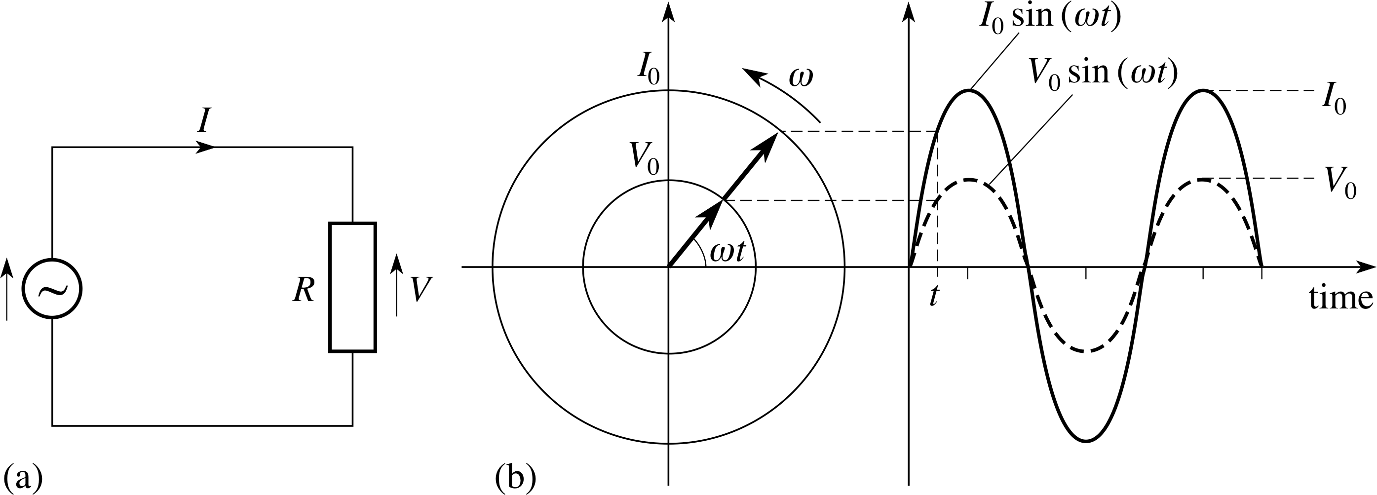
Figure 6 (a) A circuit supplying an alternating voltage (represented by the wavy line in a circle) across a resistor. The arrows shows the positive direction for the voltages, with an arrowhead at the positive end. (b) The current produced in the circuit is in phase with the voltage that causes it, as shown by the graph and the corresponding phasor diagram.
Figure 6a shows a simple a.c. circuit that supplies an alternating voltage V (t) = V0 sin(ωt) across a resistor.
Since Ohm’s law V = IR can be applied at any instant, we can expect that the varying voltage will produce a varying current given by
$I(t) = \dfrac{V(t)}{R} = \dfrac{V_0}{R}\sin(\omega t)$ i
so, if we define
$I_0 = \dfrac{V_0}{R}$(9)
then we can write
I (t) = I0 sin(ωt)(10)
A graph of this current, and the voltage that caused it, is shown in Figure 6b, along with the corresponding current and voltage phasors at an arbitrary time t. The peak current I0 has been chosen for graphical convenience in Figure 6b; in practice it would be determined by the values of V0 and R. The main point to notice about Figure 6b is that the current and the voltage rise and fall together, neither one leads or lags the other so there is no phase difference, and we can say that they are in phase. This is also clear from the phasors which rotate together, one on top of the other.
Alternating current in capacitors
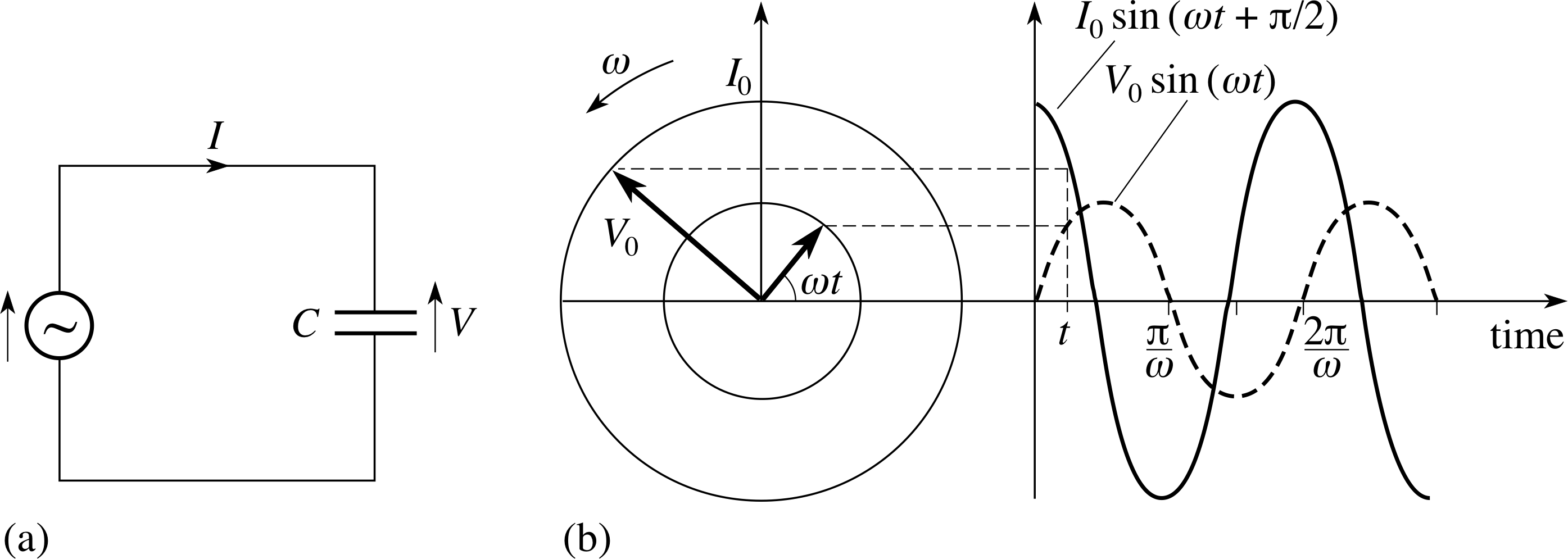
Figure 7 (a) A circuit supplying an alternating voltage across a capacitor. (b) The current produced in the circuit leads the voltage that causes it by π/2, as shown by the graph and the corresponding phasor diagram. As in Figure 6, the inner circle in part (b) represents the peak voltage V0.
A capacitor acts to store charge, and may generally be thought of as a pair of parallel conducting plates holding charges of equal magnitude but opposite sign. An alternating voltage V (t) = V0 sin(ωt) may be applied across a capacitor of fixed capacitance C by means of a circuit like that shown in Figure 7a.
No conduction current actually passes through the capacitor in such a circuit but there is an ebb and flow of charge from the capacitor as it is alternately charged and discharged; it is this flow that constitutes the current in the circuit. i
Predicting this current is a slightly indirect process but the general approach is the same as before; we start with a result that can be expected to apply at any particular instant. In the case of a capacitor, the formula that we need is that which relates the charge q stored on the capacitor to the potential difference V across it: q = CV. Assuming this is true at every instant we can write
q (t) = CV (t) = CV0 sin(ωt)(11)
Note that our (arbitrary) choice of direction for the arrow indicating the positive sense of voltages across the capacitor in Figure 7a means that the stored charge q (t) must be interpreted as the charge on the upper plate of the capacitor. Whenever V (t ) is negative (implying that the upper plate is at the lower potential), q (t) will also be negative.
Now, the current at any point in a circuit is determined by the rate of flow of charge at that point in the circuit. In Figure 7a the positive direction assigned to the current is such that a positive current will cause q (t) to increase. So, using the derivative notation of differential calculus, we find
$I(t) = \dfrac{dq(t)}{dt}$(12)
Combining this with Equation 11 gives
$I(t) = \dfrac{d[CV_0\sin(\omega t)]}{dt}$
This derivative can be easily evaluated by using the techniques of differentiation (or laboriously evaluated by drawing a graph of sin(ωt) and evaluating its gradient at many values of t). Using either method, the result will be
I (t) = ωCV0 cos(ωt)
so if we define I0 = ωCV0(13)
then we can write I (t) = I0 cos(ωt)(14)
which can be rewritten in terms of a sine function as
$I(t) = I_0\sin\left(\omega t + \dfrac{\pi}{2}\right)$(15)
Having expressed the current in terms of a sine function it is easy to see that in a circuit containing just a capacitor the current and the voltage are not in phase. The current leads the voltage by π/2. Figure 7b shows this relationship in graphical form, along with the associated phasors. As you can see the current phasor and the voltage phasor rotate at the same rate, but the current phasor is 90° ahead of the voltage phasor.
Alternating current in inductors
An inductor is essentially a coil of wire. When a current is made to flow through an inductor a magnetic field is produced in the coil.
When the current is changed, the changing magnetic flux in the coil causes an induced voltage in the coil (Faraday’s law) and the polarity of this voltage acts to oppose any change in the current.
Figure 8a shows a simple circuit that applies an alternating voltage V (t) = V0 sin(ωt) across an ideal inductor. i As the voltage changes the current will also tend to change. If the derivative dI/dt represents the rate of change of the current I (t) passing through the inductor then the size of the voltage drop across the inductor at any instant will be
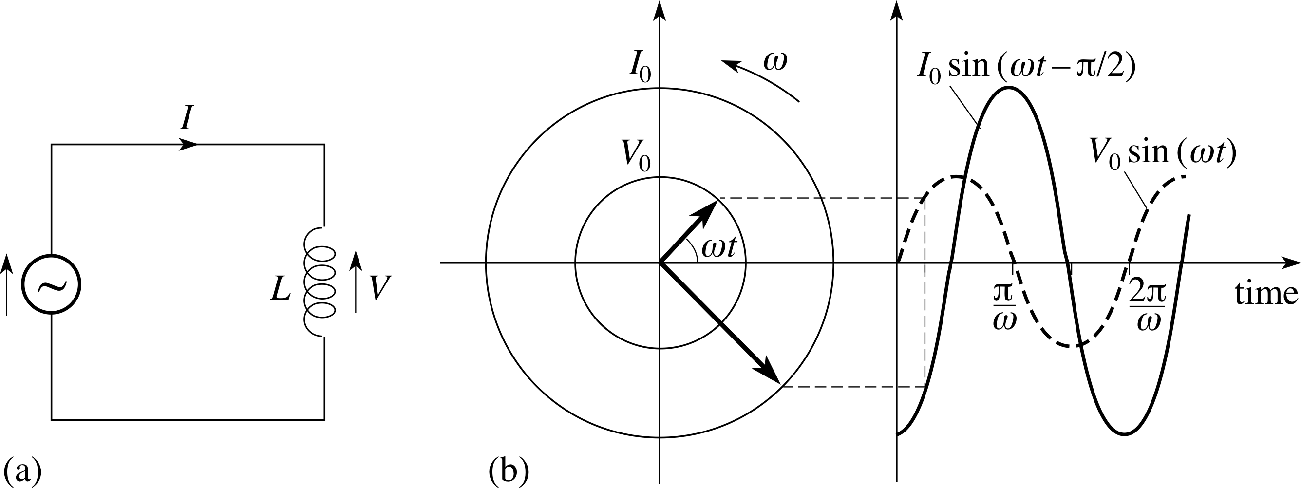
Figure 8 (a) A circuit supplying an alternating voltage across an inductor. (b) The current produced in the circuit lags the voltage that causes it by π/2, as shown by the graph and the corresponding phasor diagram.
$V(t) = L\dfrac{dI}{dt}$(16)
where the constant L is called the inductance of the inductor. You should be able to see from Equation 16 that the inductance can be expressed in units of V s A−1; such a unit is called a henry (H), so 1 H = 1 V s A−1. Widely used inductances vary from a few microhenry to hundreds of henry.
Since V (t) = V0 sin(ωt) Equation 16 gives
$\dfrac{dI}{dt} = \dfrac{V_0}{L}\sin(\omega t)$(17) i
Aside Because inductors act to oppose changes in the current they are often said to be a source of back voltage i which counters any change in the voltage supplied. Since the total voltage around a closed circuit must be zero (Kirchhoff’s voltage law) it follows that
supply voltage + back voltage = 0
If the supply voltage is given by V (t), it follows from Equation 16 that the back voltage is
induced voltage = $-L\dfrac{dI}{dt}$
Equation 17 is an example of a differential equation since it involves the derivative dI/dt of the quantity that interests us, the varying current I (t). The techniques needed to solve such equations are taught elsewhere in FLAP but you are not required to know them in order to study this module. Whenever such equations arise in this module we will simply quote their solutions and leave it to you to check by substitution that they are correct, should you wish to do so.
The solution to Equation 17, subject to the condition that there is no source of steady current in the circuit, is
$I(t) = -\dfrac{V_0}{\omega L}\cos(\omega t)$
so, if we define $I_0 = \dfrac{V_0}{\omega L}$(18)
then we can write I (t) = −I0 cos(ωt)
which we can rewrite in terms of a sine function as
$I(t) = I_0\sin\left(\omega t - \dfrac{\pi}{2}\right)$(19)
Having expressed the current in terms of a sine function we can again determine its phase relationship to the applied voltage V (t). In this case the current lags the voltage by π/2. Figure 8b shows this relationship in graphical form, along with the associated phasors. Note that the current phasor is 90° behind the voltage phasor.
Summing-up
As the above investigations show, when an alternating voltage V (t) is applied across a resistor, a capacitor or an inductor the resulting current has the same frequency as the applied voltage but is not necessarily in phase with it. In the case of the resistor the phases do coincide, but in the capacitor the current leads the voltage by π/2, and in the inductor the current lags the voltage by π/2. i
The peak value of the current, I0, depends on the resistance, capacitance or inductance in each respective case, but in addition, it also depends on the frequency of the supply in the case of a capacitor or an inductor. We will say more about this relationship in the next subsection.
✦ In each of the cases considered above we defined a quantity I0 which was interpreted as the peak current: I0 = V0/R, I0 = V0ωC and I0 = V0/(ωL). Confirm that the quantity on the right–hand side of each definition can be expressed in units of ampere (A).
✧ In each case the unit of V0 will be the volt (V). Since R is measured in ohm (Ω) and 1 Ω = 1 V A−1, it follows that V0/R may be measured in units of V/(V A−1) = A. Similarly, since the unit of ω is s−1 and that of C is the V s−1 (A s V−1) = A. Also, since L is measured in henry (H) and 1 H = 1 V s A−1, it follows that V0/(ωL) may be measured in units of V/(s−1 V s A−1) = A.
2.4 Resistance, reactance and impedance
The discussion of alternating currents in resistors in the last subsection shows no real surprises. In particular, if we measure the peak value V0 of the voltage across a resistor and the peak value I0 of the current that it causes to flow through the resistor (or the corresponding rms values), then we can easily determine the resistance R. It is given by
$R = \dfrac{V_0}{I_0} = \dfrac{V_{\rm rms}}{I_{\rm rms}}$
This resistance does not depend on the frequency of the a.c. supply and does not give rise to any phase difference between the voltage and the current.
In a similar way, we can use the quantity V0/I0 to define a sort of ‘effective a.c. resistance’ for capacitors and inductors. However, for these components the value of V0/I0 does depend on the frequency of the supply and there will be a phase difference between the voltage and the current. Since the response of capacitors and inductors depends on the nature of the supply they are said to be reactive components, and V0/I0 is called the reactance of a capacitor or an inductor, rather than its ‘resistance’. Nonetheless, the unit of reactance, like that of resistance, is still the ohm (Ω).
Using the symbols XC and XL to represent, respectively, the reactance of a capacitor and an inductor we see from Equations 13 and 18
I0 = ωCV0(Eqn 13)
$I_0 = \dfrac{V_0}{\omega L}$(Eqn 18)
(together with the relation ω = 2πf) that
$X_C = \left(\dfrac{V_0}{I_0}\right)_{\rm cap}= \dfrac{1}{\omega C}$(20)
and$X_L = \left(\dfrac{V_0}{I_0}\right)_{\rm ind} = \omega L$(21)
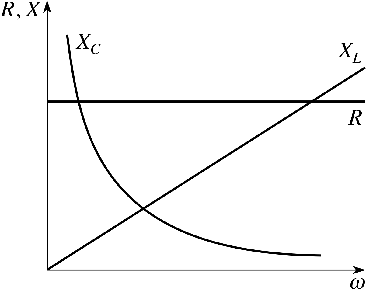
Figure 9 Graphs of R, XC and XL plotted as a function of angular frequency ω.
These results, along with the relevant phase relationships, are summarized in Table 1. Graphs showing how resistance and reactance vary with angular frequency are shown in Figure 9.
| Component | Resistance/reactance | Phase relationship |
|---|---|---|
| resistor | R = V0/I0 (constant) | V and I in phase |
| capacitor | XC = 1/(ω C) | I leads V by π/2 |
| inductor | XL = ω L | I lags V by π/2 |
✦ Figure 9 indicates that the value of R is greater than the common reactance at which XL = XR. Must this always be the case, or does it depend on the particular resistors, capacitors and inductors we choose to consider?
✧ The three curves shown in Figure 9 have no direct connection with one another. They have been plotted on a single set of axes simply to save space.
There is no reason why the values of R, C and L should be related in any way whatsoever, and therefore no reason to expect that the value of R will generally be greater than the common reactance. It is worth noting, however, that for any given values of C and L there will always be some particular frequency at which XC = XL.
We can summarize this in words by saying that the frequency does not affect the conduction through a resistor but the conduction through a capacitor increases with frequency while that through an inductor decreases with frequency. For direct current the reactance of a capacitor becomes infinite while that for an inductor falls to zero. At very high frequencies the inductor reactance rises without limit while that for the capacitor falls to zero. Inductors tend to block high frequency currents while capacitors block d.c. currents.
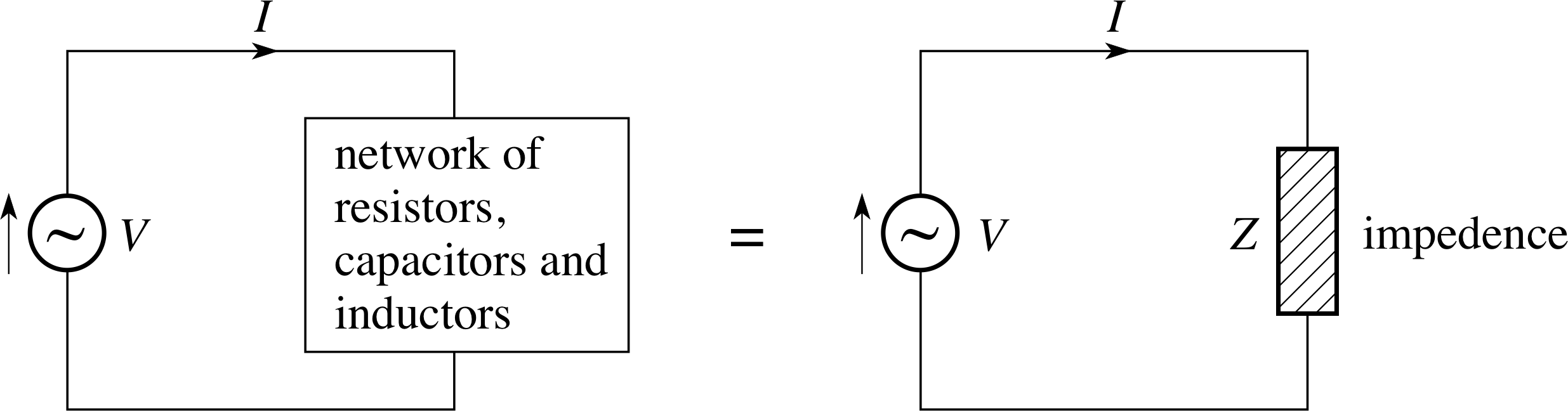
Figure 10 When a network of resistors, capacitors and inductors (with two external connections) is attached to a source of alternating voltage the effect is equivalent to that of a ‘load’ of impedance Z which causes the current to lead the voltage by a fixed phase difference ϕ.
Resistance and reactance are both special cases of a more general a.c. phenomenon known as impedance. If, as in Figure 10, an alternating voltage V (t) = V0 sin(ωt) is applied to some general network of resistors, capacitors and inductors then the current I (t) that the network draws from the supply will have the general form I (t) = I0 sin(ωt + ϕ), where I0 represents the peak value of the current and ϕ determines the phase relationship between the voltage and the current.
The values of I0 and ϕ will depend on the resistances and reactances of the various components of the network, but in general terms we say that the impedance Z of the network is
$Z = \dfrac{V_0}{I_0} = \dfrac{V_{\rm rms}}{I_{\rm rms}}$(22)
If the network consisted of a single resistor, its impedance would simply be the resistance of that resistor and ϕ would be zero. Similarly, if the network consisted of a single capacitor or inductor then its impedance would equal the reactance of that capacitor or inductor and the value of ϕ would be +π/2 or −π/2, respectively.
In the next two subsections we will investigate the impedances and phase relationships that arise from more complicated networks.
It is important to note that the instantaneous power supplied to the network in Figure 10 is given by
P (t) = V (t) I (t) = V0 sin(ωt) I0 sin(ωt + ϕ)
In the case of a resistor (or even a network of resistors), where the phase difference ϕ = 0, we have already seen that the average a.c. power over a full period (T = 2π/ω) is $\langle P\rangle = V_0I_0/2 = V_{\rm rms}I_{\rm rms}$. However, for a network containing capacitors and inductors ϕ will not generally be zero and it may be shown that
$\langle P\rangle = V_{\rm rms}I_{\rm rms}\cos\phi$(23) i
It follows that both the instantaneous and average power dissipated when the network consists of a single capacitor or a single inductor is zero since ϕ = π/2 in these cases, and cos(π/2) = 0.
✦ Express $\langle P\rangle$ for a network in terms of the impedance Z and the peak current I0, and hence show that $\langle P\rangle = I_{\rm rms}^2Z\cos\phi$.
✧ $\langle P\rangle = V_{\rm rms}I_{\rm rms}\cos\phi = (V_0I_0/2)\cos\phi = (I_0^2Z/2)\cos\phi = I_{\rm rms}^2Z\cos\phi$
It is also true that for any network consisting only of pure inductors and capacitors, there is no power dissipation, since in each component the current and voltage are 90° out of phase. Power dissipation requires the presence of resistance in the circuit.
2.5 The series LCR circuit
Combining C and R
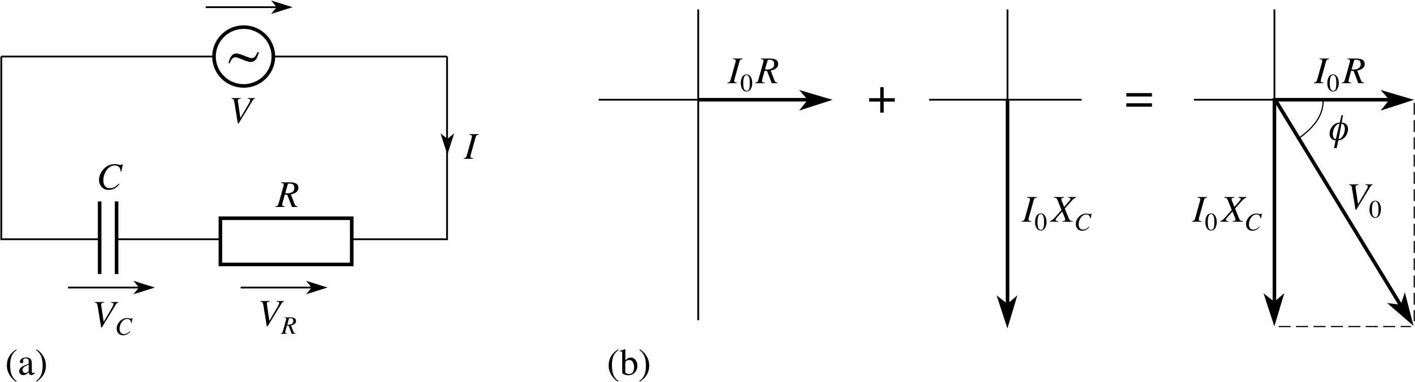
Figure 11 A capacitor and resistor in a series a.c. circuit (an RC circuit). The voltage phasors at t = 0 are shown, as is their sum which represents the total voltage that must be supplied at t = 0.
Figure 11 shows a capacitor and a resistor connected in series. When circuit components are connected in this way the same current I (t) flows through each of them, but the total instantaneous voltage V (t) across them is the sum of the instantaneous voltages VR(t) and VC(t) across the individual components. (To this extent they behave like d.c. circuits.) Since the voltage across the resistor is in phase with the current while that across the capacitor is not, it follows that the voltage across the capacitor cannot be in phase with the voltage across the resistor. This means that the total voltage across the resistor and capacitor, which is just the applied voltage V (t), will not be in phase with the voltage across either component. Nor therefore can the applied voltage be in phase with the current in the circuit.
In what follows we are going to determine the relationship between the applied voltage and the current in this circuit, which will involve finding expressions for the ratio of their peaks Z = V0/I0 and for the phase difference ϕ between them.
The easiest way to find the relationship between the peak voltages (and this is the key to finding the impedance) is to use phasor diagrams of the kind introduced in Subsection 2.1. Those needed in this case are also shown in Figure 11b. If the current is assumed to be of the form I (t) = I0 sin(ωt), then at t = 0 it can be represented by a horizontal phasor. i The voltage across the resistor VR(t) is in phase with this current so it too can be represented by a horizontal phasor at t = 0. This voltage phasor is shown in Figure 11b, it has amplitude I0R.
Now, remembering that the voltage across a capacitor lags the current through it by π/2 (since the current leads the voltage by π/2) we see that at t = 0, the voltage across the capacitor is represented by a phasor that points vertically downwards. This phasor is also shown in Figure 11b, and has amplitude I0XC, where XC is the reactance of the capacitor. The phasor representing the total voltage across the resistor and capacitor at t = 0 is obtained by adding the other two phasors together as though they were vectors. Using Pythagoras’s theorem, the amplitude V0 of this resultant phasor, which represents the total voltage across the circuit, is given by
$V_0^2 = I_0^2R^2 + I_0^2X_C^2\quad\text{i.e.}\quad V_0^2 = I_0^2(R^2 + X_C^2)$
so$V_0 = I_0\sqrt{\smash[b]{R^2 + X_C^2}}$
It follows that the impedance Z = V0/I0 of the series combination of a resistor and a capacitor is given by
$Z = \sqrt{\smash[b]{R^2 + X_C^2}}$(24)
It can also be seen from Figure 11 that the total voltage lags the voltage in the resistor by ϕ.
If we take the current phase as our reference zero then the voltage phase lag ϕ is given by
$\tan\phi = -\dfrac{X_C}{R}$
so$\phi = -\arctan\left(\dfrac{X_C}{R}\right)$(25)
Since the voltage in the resistor is in phase with the current in the circuit, and since we chose to represent the current by I (t) = I0 sin(ωt), it follows that we can represent the total voltage by V (t) = V0 sin(ωt + ϕ).
So, in a series RC circuit, the impedance is $\sqrt{\smash[b]{R^2 + X_C^2}}$, and the current leads the applied voltage by $\arctan\left(\dfrac{X_C}{R}\right)$, since ϕ is a negative quantity in this case. i
Combining L and R
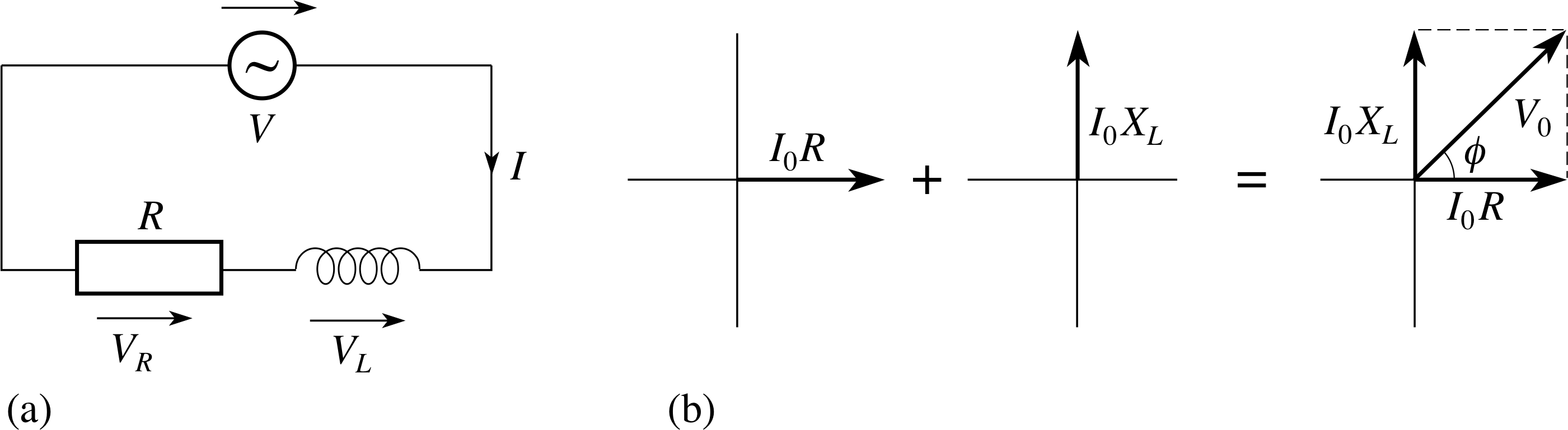
Figure 12 A resistor and an inductor in a series a.c. circuit (an LR circuit). The voltage phasors at t = 0 are shown, as is their sum which represents the total voltage that must be supplied at t = 0.
The same thing can be done for a series combination of an inductor and a resistor – which is actually how a real inductor would behave.
The relevant circuit is shown in Figure 12. Once again it will be assumed that the current is of the form I (t) = I0 sin(ωt) and as before we will write the applied voltage as V (t) = V0 sin(ωt − ϕ). The challenge is to find the ratio V0/I0 and the value of ϕ that are appropriate to this case. Of course, V0/I0 can always be written as Z, so the first problem is to find the impedance Z of the series combination. We will use the voltage phasors at t = 0 to help solve this problem.
The current in each series component is the same, and the voltage across the resistor is in phase with that current, so at t = 0 the phasor for the voltage across the resistor is horizontal and points to the right. The voltage across an inductor leads the current through it, so the phasor for the voltage across the inductor points vertically upwards in this case. The phasor representing the total voltage is the (phasor) sum of these two, as indicated in Figure 12.
Following a similar argument to that used earlier, the impedance of the LR combination will be
$Z = \sqrt{\smash[b]{R^2 + X_L^2}}$(26)
In this case the current (which is in phase with the resistor voltage) lags the total voltage. So V (t) = V0 sin(ωt + ϕ) where in this case ϕ must be a positive quantity.
$\tan\phi = \dfrac{X_L}{R}$
or equivalently $\phi = \arctan\left(\dfrac{X_L}{R}\right)$(27)
So, in a series LR circuit, the impedance is $\sqrt{\smash[b]{R^2 + X_L^2}}$ and the current lags the applied voltage.
Combining L, C and R
Figure 13 A series LCR a.c. circuit with the relevant phasor diagram showing how the individual voltages are combined. (In this case XC > XL).
Figure 13 shows a resistor, a capacitor and an inductor combined in a series a.c. circuit. The current in each component is the same and so has the same phase. It is sensible to take this current as defining our phase zero, with the voltages across each component having phase angles with respect to the current phase. This time we must add together three voltage phasors at t = 0. Fortunately two of them point in opposite directions along the same line, so their resultant is easy to determine, and this can be combined with the third phasor in the usual way.
Thus$V_0^2 = I_0^2R^2 + I_0^2(X_L-X_C)^2$
i.e.$V_0^2 = I_0^2\left[R^2 + (X_L-X_C)^2\right]$
but the impedance Z is given by Z = V0/I0, hence
the impedance of a series LCR circuit is given by
$Z = \sqrt{\smash[b]{R^2 + (X_L-X_C)^2}}$(28)
Substituting for the reactances (XL = ωL and XC = 1/(ωC)) gives us
$Z = \sqrt{R^2 + \left(\omega L -\dfrac{1}{\omega C}\right)^2}$(29)
It is also true that Z 2 = R2 + X 2 where X is the total reactance of the circuit. So, for a series circuit
(impedance)2 = (resistance)2 + (reactance)2
The constant ϕ that determines the phase relationship between the current in the circuit and the supply voltage can also be deduced from the final phasor diagram in Figure 13.
The value of ϕ is given by
$\phi = \arctan\left(\dfrac{X_L-X_C}{R}\right)$(30) i
So, in a series LCR circuit, if X C is greater than XL then ϕ will be negative and the current in the circuit will lead the total voltage (as shown in Figure 13). However, if XC is less than X L, Equation 30 will yield a positive value for ϕ, this corresponds to the case in which the current lags the total voltage.
In this convention we are taking the conventional voltage in the resistor to define the zero phase condition, so I (t) = I0 sin(ωt) and the voltage applied to the whole circuit is then V (t) = V0 sin(ωt + ϕ), where V0 = ZI0 and ϕ is given by Equation 30.
Question T3
A series LCR circuit has a supply current I (t) = I0 sin(2πft) where = 0.1 A and the supply frequency f = 50 Hz. If the components have values R = 100 Ω, C = 50 μF (i.e. 50 × 10−6 F) and L = 0.5 H, calculate the impedance of the circuit and hence obtain an expression for the supply voltage.
Answer T3
The impedance is given by Equation 28 or 29,
$Z = \sqrt{\smash[b]{R^2 + (X_L-X_C)^2}}$(Eqn 28)
$Z = \sqrt{R^2 + \left(\omega L -\dfrac{1}{\omega C}\right)^2}$(Eqn 29)
$Z = \sqrt{(100)^2 + \left(2\pi\times50\times0.5-\dfrac{1\times10^6}{2\pi\times50\times50}\right)^2}\,\Omega = 137\,\Omega$
The phase constant ϕ that determines the amount by which I (t) leads V (t) is given by Equation 30,
$\phi = \arctan\left(\dfrac{X_L-X_C}{R}\right)$(Eqn 30)
$\phi = \rm \arctan\left(\dfrac{2\pi\times50\,Hz\times50\,H-\dfrac{1}{2\pi\times50\,Hz\times0.5\,\mu F}}{100\,\Omega}\right) = +0.75\,radians$
(If you are using a calculator, use the radian mode.)
The positive value of ϕ indicates that V (t) leads I (t) in this case.
The peak of the supply voltage can be written V0 = ZI0, so the supply voltage can be expressed as
V (t) = (137 Ω)(0.1 A) sin(2πft + 0.75)
i.e.V (t) = 13.7 sin(2πft + 0.75) V
2.6 The parallel LCR circuit
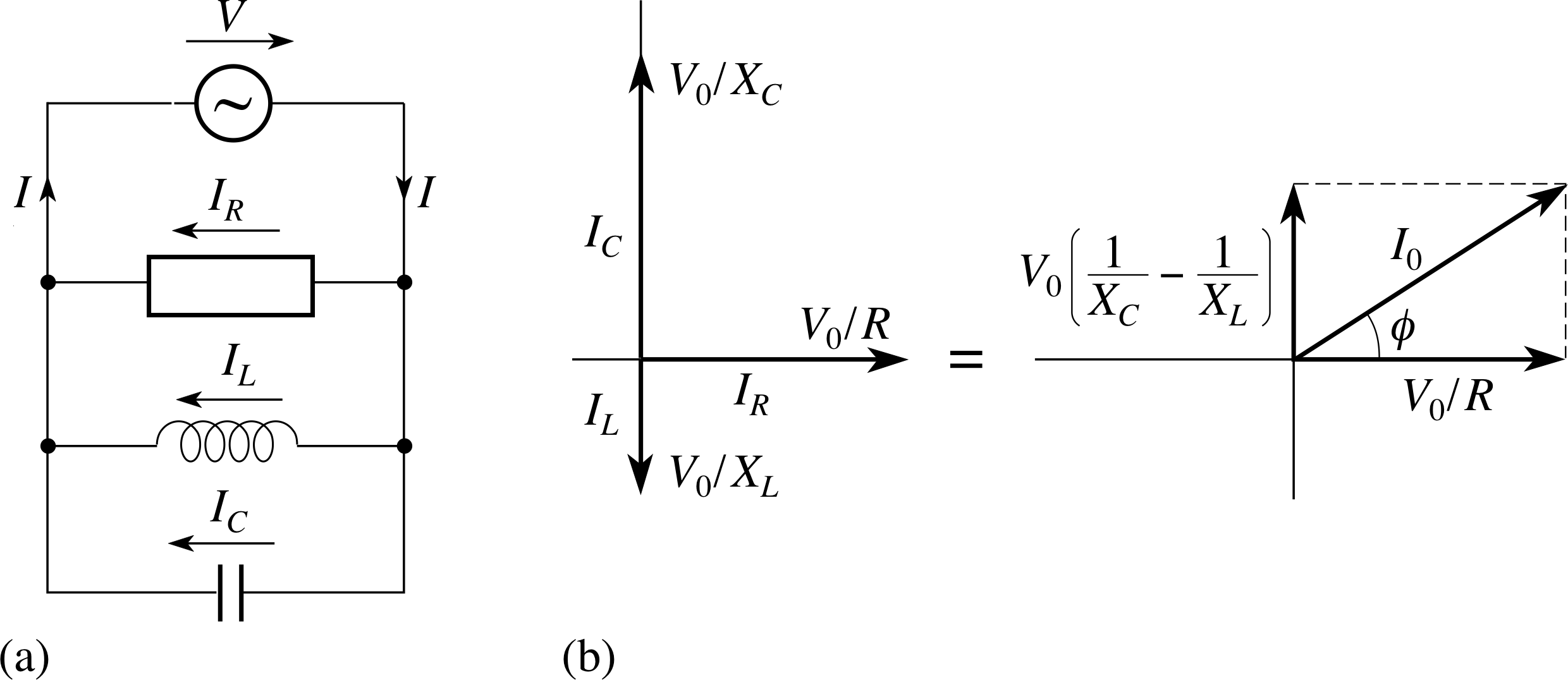
Figure 14 A parallel LCR circuit, the current phasors at t = 0, and the resultant phasor that represents the current drawn from the supply.
The basic principle that underlies the analysis of a parallel LCR circuit, of the kind shown in Figure 14 is that the instantaneous voltage V (t) is the same across each element but the current will generally differ from one component to another. When dealing with a series circuit, a phasor diagram was used to combine the voltages across currents through each component, but with a parallel circuit, phasors must be used to combine currents through each component. The total current being supplied to the combination of resistor, capacitor and inductor will therefore be the phasor sum of the individual currents in each component. The current in the resistor IR(t) is in phase with the supply voltage V (t); the current in the capacitor IC(t) leads V (t) by π/2, and the current in the inductor IL(t) lags V (t) by π/2. i
Hence, if the supply voltage is given by V (t) = V0 sin(ωt) the currents in the resistor, capacitor and inductor at t = 0 can be represented by the phasors shown in Figure 14. These phasors may be added together (like vectors) giving a resultant phasor that represents the current I (t) drawn from the supply.
✦ In Figure 14 the amplitudes of the current phasors have been denoted by the constants V0/XC, V0/R and V0/XL. This looks rather clumsy but makes more sense than denoting them IC, IR and IL. Explain why.
✧ The symbols IC, IR and IL have already been used to represent the currents in the capacitor, resistor and inductor; these currents vary with time and are represented at any moment by the (instantaneous) vertical component of the corresponding phasor. The quantities we are interested in are the constant amplitudes of the phasors.
If we use Pythagoras’s theorem to evaluate the amplitude of the resultant phasor in Figure 14, we find that the peak value of the total current in the circuit is given by
$I_0 = \sqrt{V_0^2\left(\dfrac{1}{X_C}-\dfrac{1}{X_L}\right)^2 + \dfrac{V_0^2}{R^2}}$(31)
so$\dfrac{I_0}{V_0} = \sqrt{\left(\dfrac{1}{X_C}-\dfrac{1}{X_L}\right)^2 + \dfrac{1}{R^2}}$
but the impedance Z = V0/I0. Hence,
the impedance of a parallel LCR circuit is given by
$\dfrac{1}{Z} = \sqrt{\left(\dfrac{1}{X_C}-\dfrac{1}{X_L}\right)^2 + \dfrac{1}{R^2}}$(32)
Substituting for the reactances (XC = 1/(ωC) and XL = ωL) we can rewrite this in the equivalent form
$\dfrac{1}{Z} = \sqrt{\left(\omega C-\dfrac{1}{\omega L}\right)^2 + \dfrac{1}{R^2}}$(33)
The constant ϕ that determines the phase relationship between the total current and the current through the resistor (and hence the voltage) may also be expressed in terms of the amplitudes of the three current phasors:
$\phi = \arctan\left[\left(\dfrac{V_0}{X_C}-\dfrac{V_0}{X_L}\right)\middle/\dfrac{V_0}{R}\right]$
Dividing both the numerator (the top) and the denominator (the bottom) of this expression by V0 gives us
$\phi = \arctan\left[\left(\dfrac{1}{X_C}-\dfrac{1}{X_L}\right)\middle/\dfrac{1}{R}\right]$(34)
So, in a parallel LCR circuit, if 1/XC is greater than 1/XL, then ϕ will be positive and the current will lead the voltage, but if 1/XC is less than 1/XL, ϕ will be negative and the current will lag the voltage. In other words, if the voltage in the circuit is V (t) = V0 sin(ωt), the current will be given by I (t) = I0 sin(ωt + ϕ), where I0 = V0/Z and ϕ is given by Equation 34.
Question T4
A parallel LCR circuit has a supply voltage of the form V = V0 sin(2πft), where V0 = 100 V and the supply frequency f = 50 Hz. If the components have values R = 100 Ω, C = 50 μF and L = 0.5 H, calculate the impedance of the circuit and hence write an expression for the supply current.
Answer T4
The impedance is given by Equation 32,
$\dfrac{1}{Z} = \sqrt{\left(\dfrac{1}{X_C}-\dfrac{1}{X_L}\right)^2 + \dfrac{1}{R^2}}$(Eqn 32)
$\dfrac1Z = \sqrt{\dfrac{1}{(100)^2} + \left(\dfrac{2\pi\times50\times50}{1\times10^6} - \dfrac{1}{2\pi\times50\times0.5}\right)^2}\,\Omega^{-1}$
HenceZ = 73 Ω.
The phase constant is given by Equation 34,
$\phi = \arctan\left[\left(\dfrac{1}{X_C}-\dfrac{1}{X_L}\right)\middle/\dfrac{1}{R}\right]$(Eqn 34)
$\phi = \rm \arctan\left(\dfrac{2\pi\times50\,Hz\times50\,\mu F-\dfrac{1}{2\pi\times50\,Hz\times0.5\, H}}{\dfrac{1}{100\,\Omega}}\right) = +0.75\,radians$
So, the peak of the supply current can be written V0 = ZI0 and the supply current can be expressed as
$I(t) = \dfrac{100\sin(2\pi ft + 0.75)\,{\rm V}}{73\,\Omega}$
Therefore, I (t) = 1.4 sin(2πf t + 0.75) A.
The current leads the voltage by ϕ = 0.75 radians
2.7 Combining series and parallel circuits
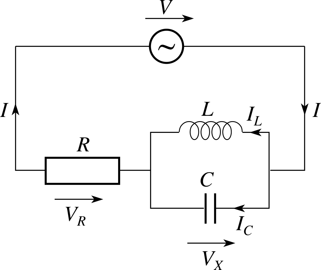
Figure 15 A circuit with a parallel combination of an inductor L and a capacitor C in series with a resistance R.
Using the rules that have been deduced above for calculating the impedance of components that are joined in series or in parallel (Equations 28 and 32, respectively)
$Z = \sqrt{\smash[b]{R^2 + (X_L-X_C)^2}}$(Eqn 28)
$\dfrac{1}{Z} = \sqrt{\left(\dfrac{1}{X_C}-\dfrac{1}{X_L}\right)^2 + \dfrac{1}{R^2}}$(Eqn 32)
it is now possible for us to work out the impedance of more complicated networks. For example, in the case of the circuit shown in Figure 15 a capacitor and an inductor are joined in parallel, and that combination is connected in series with a resistor.
According to Equation 32, the parallel part of the circuit is equivalent to a single reactance X given by
$\dfrac1X = \dfrac{1}{X_C}-\dfrac{1}{X_L}$ which implies $X = \dfrac{X_LX_C}{X_L-X_C}$
and according to Equation 28, the total impedance Z of that reactance and the resistance with which it is in series is given by
Z 2 = R2 + X 2
Thus,$Z = \sqrt{R^2 + \left(\dfrac{X_LX_C}{X_L-X_C}\right)^2}$
The voltage is the same across the inductor and the capacitor, whilst the (phasor) sum of the currents through the combination of inductor and capacitor is the same as the current through the resistor.
Question T5
A circuit like the one shown in Figure 15 has components with values R = 10 Ω, L = 50 mH and C = 500 μF. If the supply voltage has Vrms = 12 V and f = 50 Hz, calculate the impedance of the circuit and hence the currents through, and voltages across, each part of the circuit.
Answer T5
The reactances of the inductor and capacitor, respectively, are
XL = ωL = (100π) s−1 × (50 × 10−2) H = 15.7 Ω
XC = 1/(ωC) = 1/[(100π) s−1 × (500 × 10−6) F] = 6.4 Ω
So the total reactance X of the parallel part of the circuit is given by 1/X = 1/XC − 1/XL, from which X = 10.7 Ω.
The total impedance of the circuit is given by Z 2 = R2 + X 2, from which Z = 14.7 Ω.
Using V0 = ZI0, gives us I0 = 12 V/14.7 Ω = 0.82 A.
Now, the rms voltages across each part of the circuit are given by
VR,rms = IrmsR and VX,rms = IrmsX
SoVR,rms = 8.2 V and VX,rms = 8.9 V
The rms currents in the two arms of the parallel part of the circuit are given by
IC,rms = VX,rms /XC and IL,rms = VX,rms /XL
SoIC,rms = 1.39 A and IL,rms = 0.57 A
As a consistency check on these results it is worth noting that
V 2rms = V 2R,rms + V 2X,rms
which is to be expected because V (t) = VR(t) + VX(t) but VR(t) and VX(t) differ in phase by π/2.
Similarly,
Irms = IC,rms − IL,rms
which is to be expected since I (t) = IC(t) + IL(t) but IC(t) and IL(t) are out of phase by π.
2.8 Filter circuits
It is important to remember that the impedance of reactive circuit components such as capacitors and inductors depends on the (angular) frequency of the supply. This property can be put to good use in various contexts, such as the construction of filter circuits designed to block signals in certain frequency ranges while allowing others to pass. Two simple circuits of this kind R are shown in Figures 16 and 17.
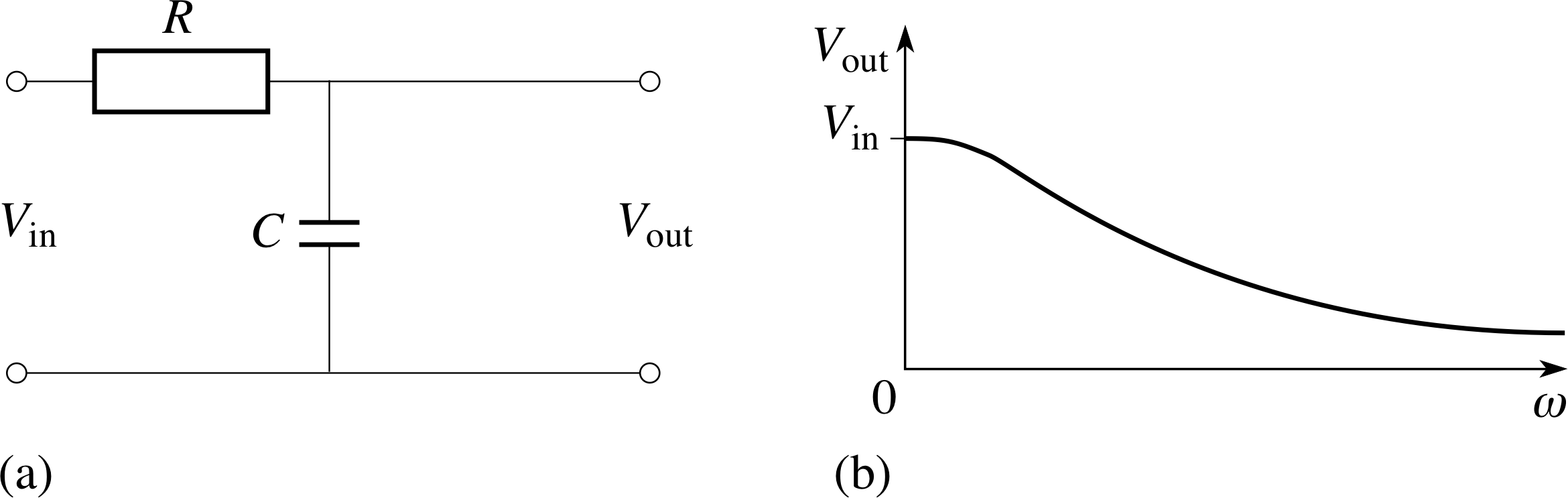
Figure 16 (a) A low–pass filter circuit. (b) Graph showing the rms output voltage as a function of the
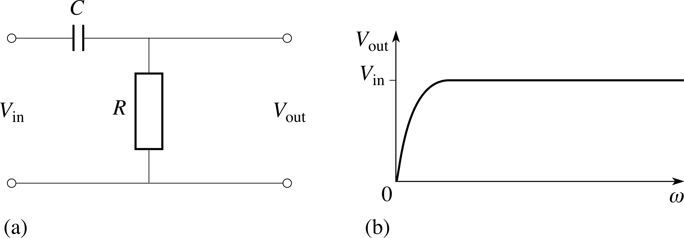
Figure 17 (a) A high–pass filter circuit. (b) Graph showing the rms output voltage as a function of the angular frequency of the input voltage.
In the case of Figure 16, an alternating supply of voltage Vin provides current to a capacitor and a resistor in series, and the varying voltage across the capacitor is used as an output voltage of rms value Vout that may supply some other circuit. The impedance of the series RC combination is $Z = \sqrt{\smash[b]{R^2 + X_C^2}}$ (Equation 12), so Vin is related to the rms current in the circuit by
$V_{\rm in} = I_{\rm rms}\sqrt{\smash[b]{R^2 + X_C^2}}$
butVout = Irms XC
so$V_{\rm out} = V_{\rm in}\dfrac{X_C}{\sqrt{\smash[b]{R^2+X_C^2}}}$
Now, this can be written in terms of angular frequency and capacitance as follows
$V_{\rm out} = V_{\rm in}\dfrac{1/\omega C}{\sqrt{\smash[b]{R^2+[1/(\omega C)]}}}$
A graph showing the rms value Vout as a function of the angular frequency ω of the supply is shown in Figure 16b.As you can see, if the input voltage has a low frequency the output voltage will have a fairly similar rms value to Vin, but if the input has a high frequency the output will have a relatively small rms value.
Thus, this particular circuit blocks high frequency signals and is therefore a crude example of a low–pass filter. You can easily imagine how useful such circuits might be in radios and other items of electrical equipment.
The next question invites you to find the formula that describes the graph in Figure 17 and hence to establish that the RC circuit shown there is an example of a high–pass filter.
Question T6
Find the rms voltage Vout for the circuit shown in Figure 17a, and confirm that its behaviour as a function of the input angular frequency is qualitatively similar to that shown in Figure 17b.
Answer T6
Following similar steps to those used in analysing the low–pass filter we find
$V_{\rm out} = V_{\rm in}\dfrac{R}{\sqrt{\smash[b]{R^2+X_C^2}}} = V_{\rm in}\dfrac{R}{\sqrt{\smash[b]{R^2+(1/(\omega C))^2}}}$
From this formula we can see that as ω approaches zero, 1/(ωC) ≫ R, and Vout approaches zero and that as ω becomes very large, 1/(ω1C) ≪ R, and Vout approaches Vin.
Moreover, when 1/(ωC)2 = 3R2, i.e. when ω = 0.58/RC,Vout = Vin /2.
This is the kind of graph shown in Figure 17b.
3 Oscillations in electrical circuits
You have now seen how capacitors and inductors respond to sinusoidal currents and voltages in a.c. circuits, but to have a more complete understanding of their behaviour you also need to know how they respond when supplies are switched on or off, or new connections are made. Such changes generally result in transients – that is brief bursts of current and voltage whose behaviour is characteristic of the component (or network of components) involved. We will temporarily return to d.c. circuits to consider this point.
3.1 Transient currents in an RC circuit
Figure 18a shows a capacitor being charged through a resistor by a d.c. supply. When the switch is first closed, at t = 0, the potential difference across the capacitor is initially zero, but it will increase with time as charge accumulates in the capacitor. This increasing potential difference VC (t) may be measured using a high impedance voltmeter (such as a cathode_rayscathode ray oscilloscope) and will change with time in the way indicated by Figure 18b.
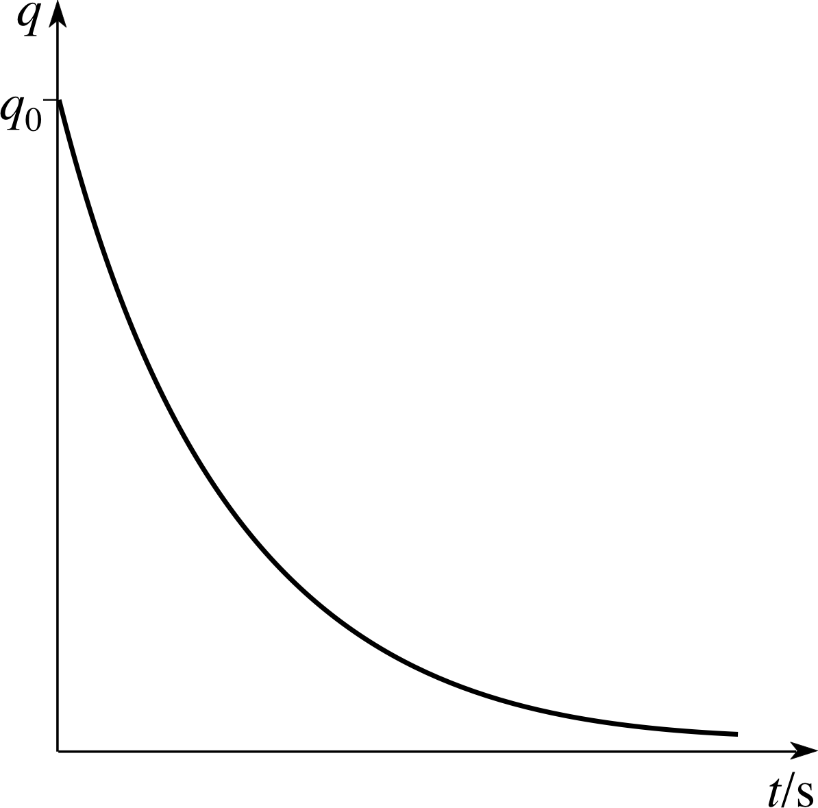
Figure 19 Discharge of a capacitor through a resistor allows the stored charge to fall from q0 to 0.
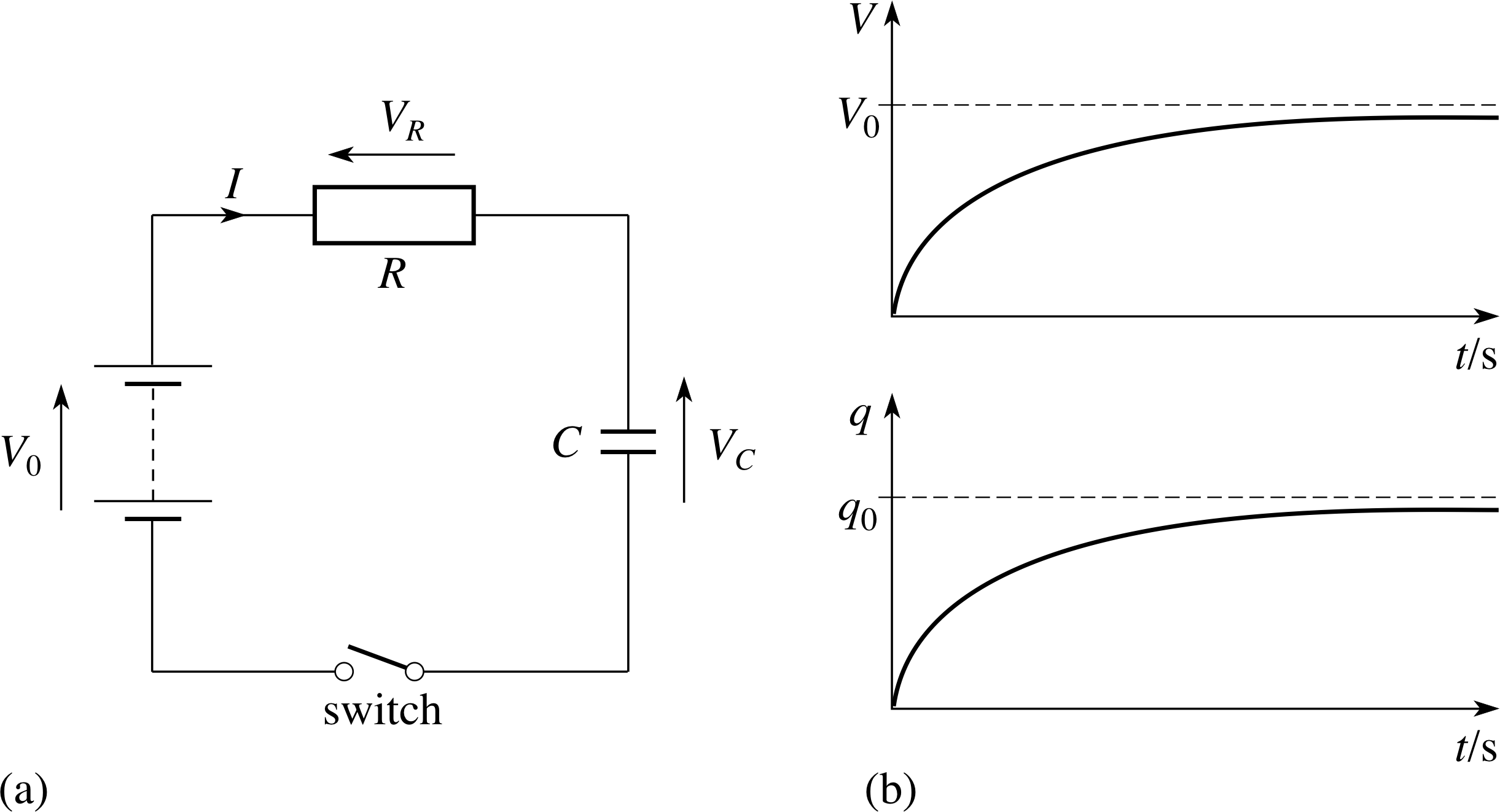
Figure 18 (a) An RC circuit for charging a capacitor through a resistor. (b) Graphs showing the change in potential difference, VC(t) and stored charge, q (t) as a function of time.
Eventually, the charge stored in the capacitor will build up to a maximum value q0 = V0C, where V0 is the voltage of the d.c. supply and C is the capacitance of the capacitor.
If the capacitor in Figure 18a is fully charged, and the battery is then replaced by a piece of wire the capacitor will discharge through the resistor. The stored charge will then decrease with time in the way shown in Figure 19.
Our aim now is to obtain the mathematical formulae that describe these curves.
Charging a capacitor
When charging the capacitor, the supplied voltage V0 must equal the sum of the voltage drops across the resistor and the capacitor at any time t.
SoV0 = VR(t) + VC(t) i
i.e.$V_0 = I(t)R + \dfrac{q(t)}{C}$
where I (t) represents the current through the resistor at time t.
Thus$I(t) = \dfrac{V_0}{R} - \dfrac{q(t)}{RC}$(35)
Now, the current I (t) is the rate of flow of charge that causes the stored charge q (t) to increase, so we can write I (t) = dq/dt. Equation 35 can therefore be rewritten as
$\dfrac{dq}{dt} = \dfrac{V_0}{R} - \dfrac{q(t)}{RC}$
i.e.$\dfrac{dq}{dt} = \dfrac{1}{RC}\left[V_0C - q(t)\right]$
Using the fact that q0 = V0C, and rearranging this last equation slightly gives us
$\dfrac{dq}{dt} = -\dfrac{1}{RC}\left[q(t) - q_0\right]$(36)
Now, R, C and q0 are all constants, so what we have here is an equation which relates q (t), the stored charge at any time t, to dq/dt, the instantaneous value of its rate of change. This is an example of a first–order differential equation, similar to the one we met in Subsection 2.3. It is said to be ‘first-order’ because it does not contain the second derivative d2q/dt2, nor any other derivative of q apart from the first derivative dq/dt. As before we will not work out the solution to the differential equation, we will just write it down and leave it to you to confirm that it is correct, should you wish to do so. In this case the general solution to the equation is
$q(t) = q_0\left[1-A\exp\left(-\dfrac{t}{RC}\right)\right]$(37) i
The arbitrary constant A that appears in this equation is a feature that arises in the general solution of every first–order differential equation. To determine its value in any particular case we must call on some appropriate item of additional information about the behaviour of q (t); some property that is not implicit in Equation 36. This additional information is called a boundary condition or an initial condition of the solution. In the case of the charging capacitor a suitable condition is the requirement that at t = 0, when charging commences, there is no stored charge in the capacitor.
In mathematical terms this means that q (0) = 0. Imposing this condition on Equation 37 (i.e. setting t = 0 and q (0) = 0) implies i
A = 1
So, the particular solution to the differential equation that is relevant to us is:
$q(t) = q_0\left[1-\exp\left(-\dfrac{t}{RC}\right)\right]$(38) i
This is the mathematical description of the charging curve shown in Figure 18b.
Figure 19 Discharge of a capacitor through a resistor allows the stored charge to fall from q0 to 0.
Figure 18 (a) An RC circuit for charging a capacitor through a resistor. (b) Graphs showing the change in potential difference, VC(t) and stored charge, q (t) as a function of time.
Discharging a capacitor
When a charged capacitor is allowed to discharge through a resistor a changing current I (t) flows through the circuit until the stored charge has been reduced to zero. In this case, since the stored charge is decreasing with time we know that its rate of change dq/dt will be negative. It follows that the current in the circuit I (t) = dq/dt will also be a negative quantity, indicating that it flows anticlockwise, in opposition to the arrow shown in Figure 18a.
Now, in the absence of a battery VR(t) + VC(t) = 0
soVR(t) = −VC(t)
But,$V_R(t) = I(t)R = \dfrac{dq}{dt}R\quad\text{and}\quad V_C(t) = \dfrac{q(t)}{C}$
Hence$\dfrac{dq}{dt} = -\dfrac{q(t)}{RC}$
Once again we have a first–order differential equation that may be solved by standard methods discussed elsewhere in FLAP. This time the general solution is
$q(t) = A\exp\left(-\dfrac{t}{RC}\right)$(39)
where A is the arbitrary constant that we expect to arise in such a solution.
The particular solution that is relevant to our problem is found by imposing the initial condition that the capacitor was charged at time q0 t = 0, so q (0) = q0. Imposing this condition we see that in this case A = q0, so
$q(t) = q_0\exp\left(-\dfrac{t}{RC}\right)$(40)
This equation shows the exponential decay expected from a discharging capacitor (Figure 19).
✦ Suppose that a capacitor is being discharged through a resistor as described above. If the charge stored on the capacitor at some particular time t1 is q1, what will be the remaining charge at time t1 + RC?
✧ From Equation 40, q (t1) = q1 exp(−t1/RC) and q(t1 + RC) = q0 exp[−(t1 + RC)/RC)]
However,
q0 exp[−(t1 + RC)/RC)] = q0 exp(−t1/RC) exp(−RC/RC) = q0 exp(−t1/RC) exp(−1)
So,
q (t1 + RC) = q (t1) exp(−1) = q1 exp(−1)
Thus, over any time interval of duration RC, the stored charge is reduced by a factor of 1/e. This is a characteristic property of exponential decay.
Now that you know how a capacitor charges and discharges, the next thing to look at is the transient currents which flow when a circuit containing a resistor and an inductor is switched on and off.
3.2 Transient currents in an LR circuit
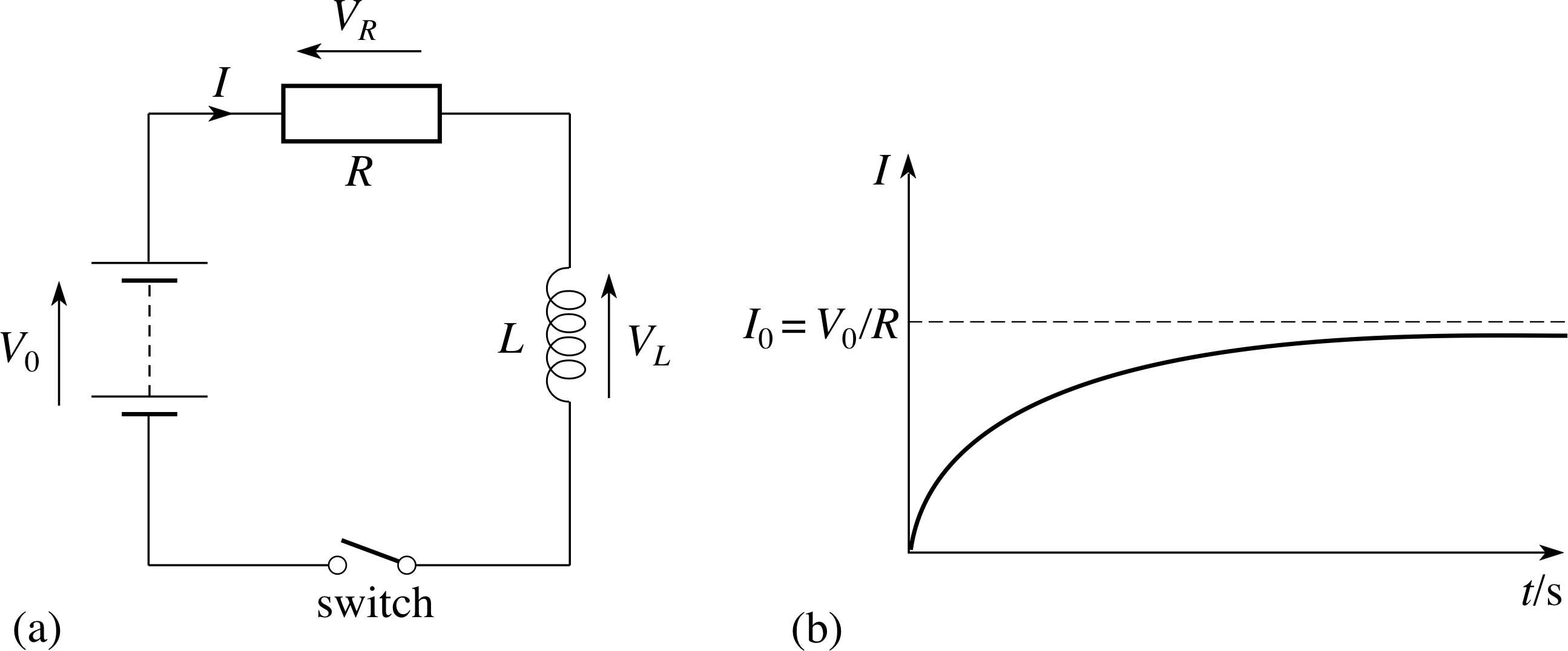
Figure 20 (a) An LR circuit for building the current through an inductor. (b) Graph showing the growth of the current as a function of time.
Figure 20a shows a resistor and an inductor connected in series to a d.c. supply of voltage V0. At any time after the switch is closed, the total voltage across the circuit is given by the sum of the V0 voltages across the individual components, so
V0 = VR(t) + VL(t)
Using Ohm’s law to find the voltage drop across the resistor and using Equation 16,
$V(t) = L\dfrac{dI}{dt}$(Eqn 16)
for that across the inductor we can rewrite this in terms of the current I (t):
$V_0 = I(t)R + L\dfrac{dI}{dt}$(41)
This can be rearranged to give
$\dfrac{dI}{dt} = -\dfrac RL\left(I(t)-\dfrac{V_0}{R}\right)$(42)
Now, when this circuit has been switched on for a sufficiently long time the current will reach a final steady value I (t) = I0. When that happens dI/dt = 0, so it follows from Equation 40,
$q(t) = q_0\exp\left(-\dfrac{t}{RC}\right)$(Eqn 40)
that I0 = V0/R.
Thus, Equation 42 may be rewritten as
$\dfrac{dI}{dt} = -\dfrac RL\left[I(t)-I_0\right]$(43)
✦ By comparing Equation 43 with Equation 36,
$\dfrac{dq}{dt} = -\dfrac{1}{RC}\left[q(t) - q_0\right]$(Eqn 36)
write down its general solution.
✧ Equations 36 and 43 are of the same form except that q has been replaced by I, and 1/RC by R/L. It follows from Equation 37,
$q(t) = q_0\left[1-A\exp\left(-\dfrac{t}{RC}\right)\right]$(Eqn 37)
that the general solution to Equation 43 must be
$I(t) = I_0\left[1-A\exp\left(-\dfrac{Rt}{L}\right)\right]$
✦ What is the value of A in this case, and what is the condition that determines it?
✧ If we require that the initial value of the current is zero (due to the opposition to change by the induced voltage of the inductor), we see that I (0) = 0.
It follows that A = 1 in this case.
The particular solution that interests us is therefore
$I(t) = I_0\left[1-\exp\left(-\dfrac{Rt}{L}\right)\right]$(44)
The transient current which flows in an inductor as the circuit is completed produces a curve similar to that in Figure 20b. Note that this curve for the growth of current in an inductor has the same overall V0 shape as the curve for the growth of stored charge in a capacitor.
If the voltage supply is replaced by a piece of wire, then the current across the inductor will decay. In that case it follows from Equation 41that
$I(t)R = -L\dfrac{dI}{dt}$(45)
Question T7
By comparing Equation 45 with that used to describe the discharge of a capacitor, and by imposing an appropriate boundary condition, show that the decaying current can be described by Equation 46 below.
Answer T7
Equation 45,
$I(t)R = -L\dfrac{dI}{dt}$(Eqn 45)
would be identical to Equation 39,
$q(t) = A\exp\left(-\dfrac{t}{RC}\right)$(Eqn 39)
if we replaced I by q, and R/L by 1/RC. It follows that the general solution to Equation 45 is
$I(t) = A\exp\left(-\dfrac{Rt}{L}\right)$
Requiring that I (t) should have had its steady state value I0 = V0/R at t = 0 implies that A = I0 in this case, so that the particular solution of interest is that given by Equation 46,
$I(t) = A\exp\left(-\dfrac{Rt}{L}\right)$(Eqn 46)
as required.
$I(t) = I_0\exp\left(-\dfrac{Rt}{L}\right)$(46)
Notice that in this case the time required for the current to decay by a factor of 1/e is L/R, so increasing the resistance will speed–up the decay.
3.3 Oscillations in LC circuits
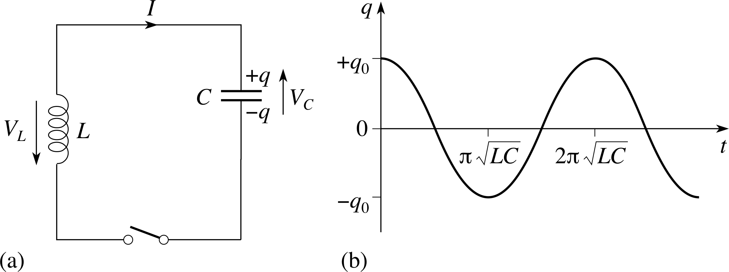
Figure 21 (a) A combination of a charged capacitor and an inductor (an LC circuit). (b) The oscillating value of the stored charge in the capacitor.
Having looked at the response of capacitors and inductors individually to transient currents and voltages, the next step is to look at how they behave when connected together, as shown in Figure 21.
In drawing the circuit, arbitrary ‘positive’ directions have been assigned to the current I (t) and the potential differences VC(t) and VL(t). i
At all times the total voltage drop around the whole circuit must be zero, so
VC(t) + VL(t) = 0
soVC(t) = −VL(t)
where$V_C(t) = \dfrac{q(t)}{C}\quad\text{and}\quad V_L(t) = L\dfrac{dI}{dt}$
Hence$L\dfrac{dI}{dt} = -\dfrac{q(t)}{C}$(47)
If the capacitor in Figure 21a initially has a stored charge q0 as shown, then, when the switch is first closed, current will flow around the circuit in the anticlockwise direction, so I (t) = dq/dt will be negative and q (t) will decrease. It follows from Equation 47 that dI/dt will be negative, causing VL(t) to be negative. This negative potential difference will counterbalance the positive (but decreasing) voltage VC(t) across the capacitor.
At all times$I(t) = \dfrac{dq}{dt}$
so$\dfrac{dI}{dt} = \dfrac{d^2q}{dt^2}$
and consequently Equation 47 may be rewritten as
$\dfrac{d^2q}{dt^2} = -\dfrac{q(t)}{LC}$(48)
Now, this is a differential equation that contains a second derivative, but no higher derivatives, so it is called a second–order differential equation.
We can simplify Equation 48 a little, or at least make it more recognizable if we rewrite it in the following way:
$\dfrac{d^2q}{dt^2} = -\omega^2 q(t)$(49) i
where$\omega_0 = \sqrt{\dfrac{1}{LC}}$(50)
The general solution to a second–order differential equation contains two arbitrary constants. If we call them A and ϕ we can write the general solution as
q (t) = A cos(ω0t + ϕ)(51)
Equation 51 indicates that q (t) oscillates with angular frequency ω0, increasing and decreasing in repetitive cycles between +A and −A, and having an initial value A cos(ϕ) when t = 0. In order to determine the arbitrary constants A and ϕ we will need two appropriate boundary conditions. The first of these is that at t = 0 the stored charge in the capacitor is q (0) = q0. The second is that this is the maximum positive value of the charge. i
The second of these conditions implies that A cos(ϕ) = A, so ϕ = 0. The first condition then implies that A cos(ϕ) = A cos(0) = A = q0. Thus, the particular solution that is of interest to us is
$q(t) = q_0\cos(\omega_0t) = q_0\cos\left(\dfrac{t}{\sqrt{LC\os}}\right)$(52)
Figure 21b The oscillating value of the stored charge in the capacitor.
The oscillations of the stored charge described by this Equation 52 are shown in Figure 21b. Note that the period of the oscillations is
$T = \dfrac{2\pi}{\omega_0} = 2\pi\sqrt{LC\os}$(53)
so the corresponding frequency is
$f_0 = \dfrac1T = \dfrac{\omega_0}{2\pi} = \dfrac{1}{2\pi\sqrt{LC\os}}$(54)
This is usually called the natural frequency of the LC circuit, and ω0 is called its natural angular frequency.
The charge oscillations described by Equation 52 cause the current in the circuit, I (t) = dq/dt, to oscillate and this causes associated oscillations in the voltages VC(t) and VL(t).
Question T8
Find the particular expressions for I (t), VC(t) and VL(t) that correspond to Equation 52,
$q(t) = q_0\cos(\omega_0t) = q_0\cos\left(\dfrac{t}{\sqrt{LC\os}}\right)$(Eqn 52)
Describe the phase relationship between each of these quantities and the stored charge q (t).
[Hint: You may find the following mathematical results useful:
$\dfrac{d}{dt}[\sin(\omega t)] = \omega\cos(\omega t),\quad\dfrac{d}{dt}[\cos(\omega t)] = -\omega\sin(\omega t)$;
$\dfrac{d}{dt}[kf(t)] = k\dfrac{d}{dt}[f(t)],$ where k is a constant.]
Answer T8
$I(t) = \dfrac{dq}{dt} = -\omega_0A\sin(\omega_0t+\phi)$
but we know that A = q0 and ϕ = 0 in this case, so:
I (t) = −ω0q0 sin(ω0t)
where$\omega_0 = 1/\sqrt{LC\os}$
VC(t) = q (t)/C = (A/C) cos(ω0t + ϕ) = (q0/C) cos(ω0t)
$V_L(t) = L\dfrac{dI}{dt} = -L\omega_0^2\cos(\omega_0t)$
To reveal the phase relationships we can re–express these results as follows
q (t) = q0 cos(ω0t)
I (t) = ω0q0 cos(ω0t + π/2)
V0(t) = (q0/C) cos(ω0t)
$V_L(t) = L\omega_0^2\cos(\omega_0t+\pi)$
So, I leads q by π/2; VC is in phase with q, and VL leads q by π.
The oscillations described in general by Equation 51,
q (t) = A cos(ω0t + ϕ)(Eqn 51)
and in particular by Equation 52,
$q(t) = q_0\cos(\omega_0t) = q_0\cos\left(\dfrac{t}{\sqrt{LC\os}}\right)$(Eqn 52)
are examples of simple harmonic oscillations.
The same sort of oscillations can be seen in the simple harmonic motion (SHM) of many mechanical systems, such as a mass on a spring or a pendulum swinging back and forth through a small angle. The capacitor in an LC circuit, with its ability to store charge, behaves to some extent like a spring, a ready source of energy. The inductor, constantly striving to prevent changes in the current, is to some extent like a mass, always reluctant to be accelerated.
As the charge in an LC circuit flows back and forth, the energy is ebbing and flowing between the capacitor and the inductor. At one moment in the cycle, all the energy is stored in the electric field of the capacitor. As this field decays, the energy is transferred to the inductor where it is stored in the magnetic field. As this field in turn decays, an electric field develops in the capacitor and the whole process continues its cycle. No power is dissipated in these interchanges because the voltages across the capacitor and the inductor always lead or lag the current by π/2. Thus in each case $\langle P\rangle = V_{\rm rms}I_{\rm rms}\cos\phi = 0$.
Question T9
Suppose that you have measured the currents and stored charges in an LC circuit in which the inductance is 1.00 H and the capacitance is 1.00 μF (i.e. 1.00 × 10⁻⁶ F), and that at time t = 0 you found that a current of 0.20 A flowed towards a capacitor plate that carried a charge of + 0.40 mC. Find the general expression for the current in the circuit at an arbitrary time t.
Answer T9
We know that in general:
q (t) = A cos(ω0t + ϕ)(Eqn 51)
so$I(t) = \dfrac{dq}{dt} = -\omega_0A\sin(\omega_0t+\phi)$
where$\omega_0 = 1/\sqrt{LC\os}$ and at t = 0, q (0) = A cos(ϕ) = 0.4 × 10⁻³ C
andI (0) = −Aω0 sin ϕ = 0.2 A
Thus$A\sin\phi = \rm -\dfrac{0.2\,A}{\omega_0} = -0.2\times10^{-3}\,C$
Since sin2ϕ + cos2ϕ = 1, it follows that
$A = \sqrt{\smash[b]{(A\sin\phi)^2+(A\cos\phi)^2}} = \sqrt{20\times10^{-8}}\,C = 4.5\times10^{-4}\,C$
Also, since tan ϕ = sin ϕ/cos ϕ
$\phi = \arctan{A\sin\phi}{A\cos\phi} = \arctan(-0.5)$
Now, care is needed at this point since arctan(x) is defined in such a way that its values are in the range −π/2 to π/2, but ϕ may be in the range −π to π. In order to determine the true value of ϕ we note that cos ϕ is positive and sin ϕ is negative, implying that ϕ is in the range −π/2 to 0. Thus we may simply accept the value of ϕ provided by a calculator without needing to adjust it in any way.
Thus,ϕ = arctan(−0.5) = −0.46. (If you are using a calculator, use the radian mode.)
Hence,I (t) = −0.45 sin[(103 s−1) t − 0.46] A
3.4 Damped oscillations in LCR circuits
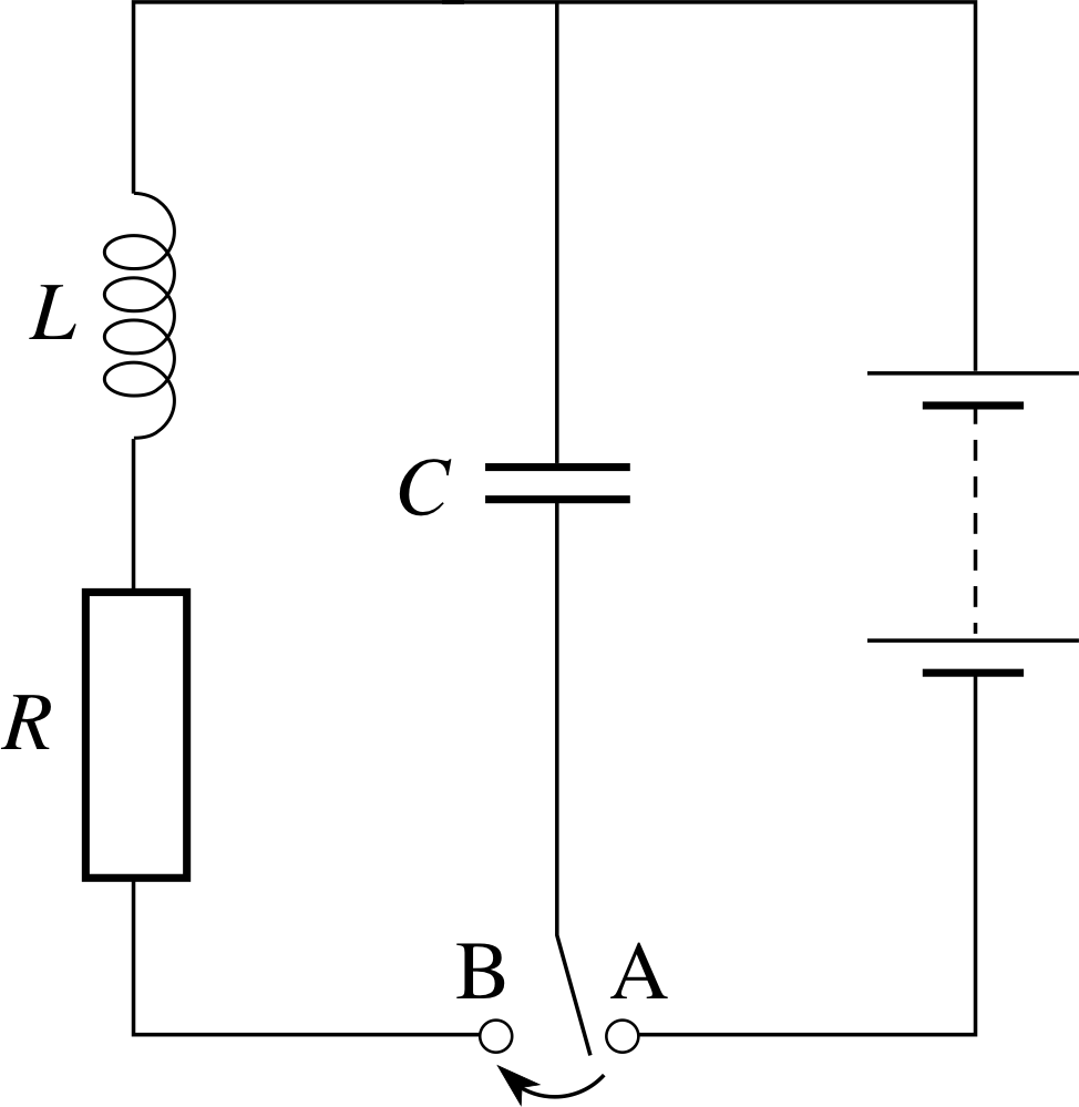
Figure 22 Circuit containing an inductor, a capacitor and a resistor. When the switch is moved from A to B the capacitor discharges through the resistor and the inductor.
The argument presented above showed that no energy is lost from an LC circuit, so the oscillations should continue for ever without any decrease in L amplitude or change of frequency. However, in reality, electromagnetic energy will be lost due to heating because real inductors always have some resistance and this will alter the phase relationship between the current and the voltage. This phenomenon of decaying oscillatory behaviour is called damping. i A more realistic circuit, containing a resistor as well as an inductor and a capacitor is shown in Figure 22. In this case the capacitor can be charged when the switch is set at A, and discharged through the inductor and the resistor when the switch is at B. i
✦ In what direction will the current flow when the switch is first moved from A to B? If q (t) represents the charge on the upper plate of the capacitor, deduce the differential equation that q (t) must satisfy.
✧ The upper plate of the capacitor will be positively charged by the battery so when the capacitor starts to discharge through the resistor and inductor the (conventional) current will initially flow in the anticlockwise direction. If we arbitrarily choose the positive direction of current flow to be clockwise (so the initial current is negative), and if we take anticlockwise to be the positive direction for voltage drops, then we can write
VC(t) + VR(t) + VL(t) = 0
where
$V_C(t) = \dfrac{q(t)}{C}$;
$V_R(t) = I(t)R = R\dfrac{dq}{dt}$;
and$V_L(t) = L\dfrac{dI}{dt} = L\dfrac{d^2q}{dt^2}$
Thus
$L\dfrac{d^2q}{dt^2} + R\dfrac{dq}{dt} + \dfrac{q(t)}{C} = 0$(55)
The general solution to this second–order differential equation for values of R2 which are less than 4L/C may be written:
$q(t) = A\exp\left(-\dfrac{Rt}{2L}\right)\cos(\omega t + \phi)$(56)
where$\omega = \sqrt{\dfrac{1}{LC} - \dfrac{R^2}{4L^2}}$(57)
As usual, boundary conditions (such as the values of q (t) and dq/dt = I (t) at some particular value of t) are required to determine the values of the arbitrary constants A and ϕ. However, irrespective of those values, provided A is not zero, it is possible to interpret Equation 56 as the mathematical description of a quantity that oscillates with angular frequency ω and with an ‘amplitude’ $A\exp\left(-\dfrac{Rt}{2L}\right)$ that decays exponentially with time.
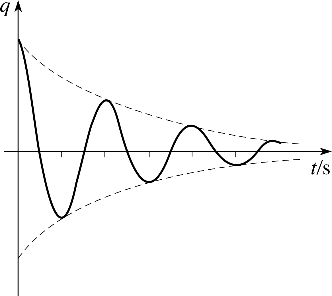
Figure 23 Damped oscillation in a series LCR circuit for which R2 < 4L/C. Note that the value of q (t) at t = 0 is related to the arbitrary constants, since q (0) = A cos ϕ.
This kind of oscillation is an example of a damped oscillation and is illustrated by the dashed line in Figure 23. Note that if we identify $1/\sqrt{LC\os}$ as the natural angular frequency ω0 in the case where R = 0, then we can write
$\omega = \omega_0\sqrt{1-\dfrac{R^2C}{4L}}$(58)
showing that the angular frequency of a damped LCR circuit is lower than the natural frequency ω0 of a pure (undamped) LC circuit.
The exponentially decaying damped oscillations that Equations 56 and 57 describe, those which arise for R2 < 4L/C, are said to exhibit underdamping. Underdamping occurs with relatively small values of R.
If R2 is very large compared with 4L/C then the capacitor takes a relatively long time to discharge and no oscillation takes place. In this case, the circuit is said to exhibit overdamping. In critical damping R2 = 4L/C and the behaviour of q (t) lies between these two extremes, with no full oscillation but, in general, with a single overshot of the q = 0 condition. i
3.5 Driven oscillations in LCR circuits
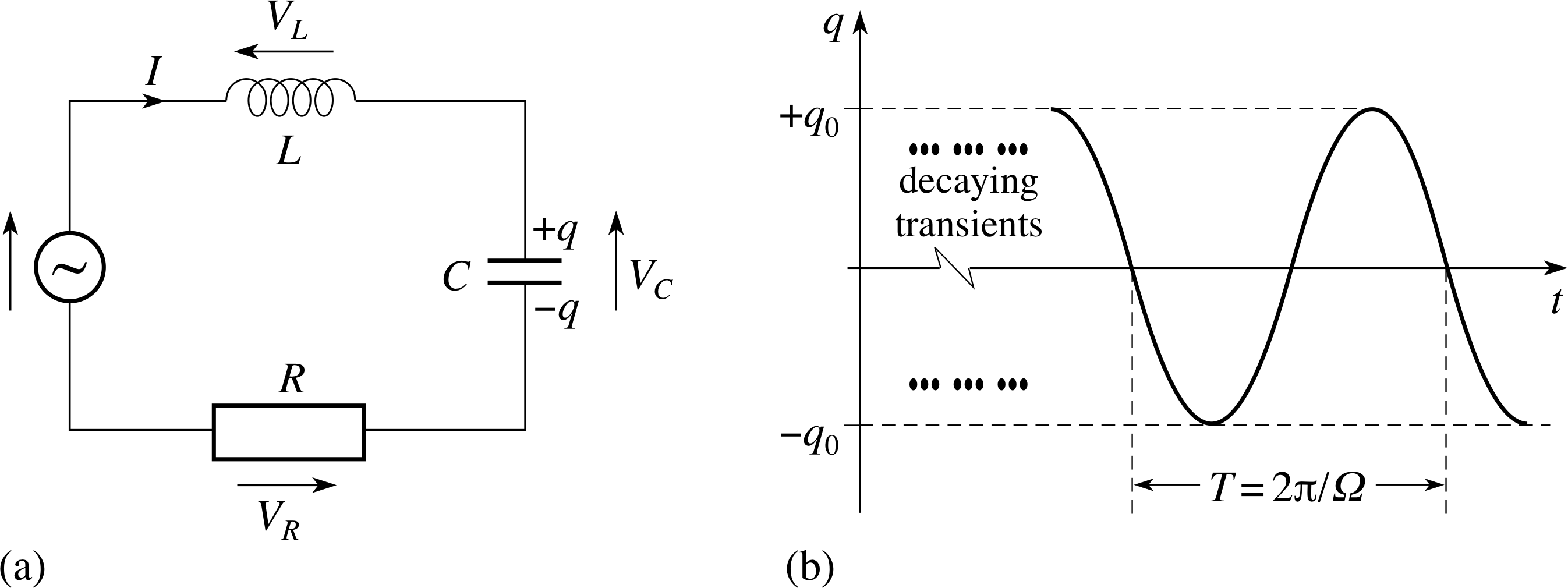
Figure 24 (a) A driven LCR circuit. (b) Graph showing the oscillatory behaviour of q (t) after any transients have died away. The current in the circuit will show similar oscillations, though their amplitude will be AΩ and they will lead the charge oscillations by π/2.
Whether they do so rapidly or slowly, oscillations in a resistive circuit (i.e. one which has a resistance) will always decay with time. However, if a supply of alternating current is made part of such a circuit it can supply the electromagnetic power that is dissipated and sustain the oscillations indefinitely. The oscillations that occur under these circumstances are called driven oscillations or forced oscillations, since their (angular) frequency will generally be that of the alternating supply rather than any ‘natural’ (angular) frequency associated with the circuit itself.
A driven LCR circuit is shown in Figure 24a.
If the a.c. supply provides an alternating voltage V (t) = V0 sin(Ωt), then the sum of the voltages around the circuit must be zero and so the stored charge q (t) must satisfy the second–order differential equation
$L\dfrac{d^2q}{dt^2} + R\dfrac{dq}{dt} + \dfrac{q(t)}{C} = V_0\sin({\it\Omega}t)$(59)
where Ω is the angular frequency of the supply.
This equation is harder to solve than those we dealt with earlier, so we will not bother to write down the general solution, we will simply round off our discussion of electrical oscillations by noting some of its main features.
The first thing to note is that after any initial transient behaviour has died away the solutions will take the form of simple harmonic oscillations described by
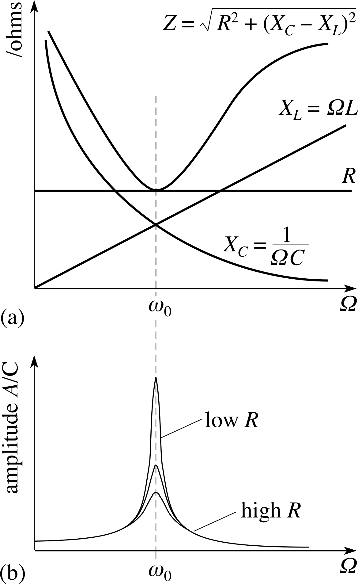
Figure 25 (a) Graphs showing the variation of reactance with angular frequency Ω. (b) A graph showing the variation of the amplitude of the oscillations with Ω.
q (t) = A sin(Ωt + ϕ)
where$A = \dfrac{V_0}{\sqrt{\smash[b]{[(1/C)-L{\it\Omega}^2]^2+(R{\it\Omega})^2}}}$
and$\phi = \arctan\left(\dfrac{-R{\it\Omega}}{(1/C)-L{\it\Omega}^2}\right)$
Notice that the amplitude A of these driven oscillations depends on Ω, the angular frequency of the a.c. supply.
A graph showing the variation of A with Ω is given in Figure 25b. As you can see the amplitude in Figure 25b,
$A = \dfrac{V_0}{\sqrt{\smash[b]{[(1/C)-L{\it\Omega}^2]^2+(R{\it\Omega})^2}}}$
shows a pronounced maximum when Ω is close to the natural angular frequency $\omega_0 = 1/\sqrt{LC\os}$. This is the phenomenon of resonance, the existence of a driving frequency which provokes an exceptionally strong response from the circuit.
Since $\omega_0 = 1/\sqrt{LC\os}$ at resonance, or very nearly, we can rewrite the approximate resonance condition as
$\omega_0L= \dfrac{1}{\omega_0C}$(60)
that is, the reactances of the inductor and capacitor are equal
XL = XC(61)
and the phase $\phi = \arctan\left(\dfrac{-R{\it\Omega}}{(1/C)-L{\it\Omega}^2}\right)$ becomes zero.
This means that the impedance of a series LCR circuit $Z = \sqrt{\smash[b]{R^2 + (X_L-X_C)^2}}$ has its minimum value, R, at resonance (see Figure 25a).
The rms current flowing in the circuit will be given by Irms = Vrms /Z, so (for a constant rms supply voltage) the rms current will be a maximum at resonance in a series LCR circuit.
Figure 14 A parallel LCR circuit, the current phasors at t = 0, and the resultant phasor that represents the current drawn from the supply.
The voltage in a parallel LCR circuit (Figure 14) shows similar resonant behaviour. In that case
$\dfrac1Z = \sqrt{\left(\dfrac{1}{X_C}-\dfrac{1}{X_L}\right)^2+\dfrac{1}{R^2}}$
so, 1/Z is a minimum at resonance. Consequently Z has its maximum value R at resonance. The rms voltage across each component is the same in this case, and is related to the rms current in the circuit by Vrms = ZIrms so (for a constant rms supply current) the rms voltage is a maximum at resonance in a parallel LCR circuit.
4 Closing items
4.1 Module summary
- 1
-
An alternating current is a flow of electric charge that reverses its direction periodically. It may be described by
I (t) = I0 sin(ωt + ϕ)(Eqn 3b)
where I0 is the amplitude or peak value of the current, (ωt + ϕ) is its phase, and ϕ is its phase constant. ω is the angular frequency of the current, which also has a period T = π/ω and a frequency f = 1/T. The root-mean-square value of such a current is given by $I_{\rm rms} = I_0/\sqrt{2}$.
- 2
-
An alternating voltage V (t) = V0 sin(ωt) applied across a resistor, a capacitor or an inductor will cause an alternating current I (t) = I0 sin(ωt + ϕ). The current through the resistor will be in phase with the voltage, so ϕ = 0. The current through the capacitor will lead the voltage by ϕ = π/2, and that through the inductor will lag the voltage by ϕ = π/2.
- 3
-
The role of impedance in a.c. circuits is analogous to that of resistance in d.c. circuits. If a voltage V (t) = V0 sin(ωt) applied across a network of components causes an alternating current I (t) = I0 sin(ωt + ϕ), the impedance of the network is given by Z = V0/I0, and the average power dissipated in the network is
$\langle P\rangle = V_{\rm rms}I_{\rm rms}\cos\phi = I_{\rm rms}^2Z\cos\phi$
- 4
-
A capacitor of capacitance C has a capacitative reactance XC = 1/(ωC) where ω is the angular frequency of the voltage supply. Similarly, an inductor of inductance L has an inductive reactance XL = ωL. The impedance of a single capacitor or inductor is equal to its reactance, the impedance of a single resistor is equal to its resistance.
- 5
-
In a series LCR circuit the total impedance is
$Z = \sqrt{\smash[b]{R^2 + (X_L-X_C)^2}}$(Eqn 28)
and the voltage leads the current b
$\phi = \arctan\left(\dfrac{X_L-X_C}{R}\right)$(Eqn 30)
In a parallel LCR circuit the total impedance is
$\dfrac{1}{Z} = \sqrt{\left(\dfrac{1}{X_C}-\dfrac{1}{X_L}\right)^2 + \dfrac{1}{R^2}}$(Eqn 32)
and the current leads the voltage by
$\phi = \arctan\left[\left(\dfrac{1}{X_C}-\dfrac{1}{X_L}\right)\middle/\dfrac{1}{R}\right]$(Eqn 34)
- 6
-
Short lived variations in current and voltage called transients can arise when the conditions in a reactive circuit are suddenly disturbed. Such transients may be studied with the aid of an appropriate first-order differential equation, relating the instantaneous value of a quantity (such as the stored charge q (t)) to its instantaneous rate of change (dq/dt). Such an equation has a general solution which contains an arbitrary constant. The general solution may be particularized to a specific physical situation by using an appropriate boundary condition to determine the value of the arbitrary constant.
- 7
-
In an LC circuit consisting of an capacitor connected to an inductor, the stored charge will exhibit simple harmonic oscillations described by
q (t) = A cos(ω0t + ϕ)
where A and ϕ are arbitrary constants with values that must be determined from appropriate boundary conditions and the natural angular frequency
$\omega_0 = \sqrt{\dfrac{1}{LC}}$(Eqn 50)
Such oscillations satisfy a characteristic second–order differential equation which may be written in the form
$\dfrac{d^2q}{dt^2} = -\omega^2 q(t)$(Eqn 49)
- 8
-
The addition of a series resistor to an LC circuit results in an LCR circuit in which, under appropriate conditions, the stored charge exhibits damped oscillations in which the ‘amplitude’ decays with time. The frequency of these oscillations is less than the natural frequency of the corresponding undamped LC circuit.
- 9
-
The further addition of an alternating voltage supply to the LCR circuit eventually results in driven oscillations of the stored charge that have the same angular frequency as the supply. The amplitude of such oscillations is a function of the supply frequency and is strongly peaked when the supply frequency is close to the natural frequency of the corresponding LC circuit. The ability of a supply of appropriate frequency to excite large amplitude oscillations in the stored charge (and the current) is an example of the phenomenon of resonance.
4.2 Achievements
Having completed this module, you should be able to:
- A1
-
Define the terms that are emboldened and flagged in the margins of the module.
- A2
-
Describe alternating currents and voltages in terms of sinusoidal functions.
- A3
-
Characterize sinusoidally varying quantities in terms of their root-mean-square values and use those values in calculating power dissipation in simple a.c. circuits.
- A4
-
Calculate the reactance of inductors and capacitors.
- A5
-
Use phasor diagrams to determine current, voltage, impedance and phase in series and parallel LCR circuits, and in simple combinations of series and parallel LCR circuits.
- A6
-
Describe the transient behaviour of stored charge (and consequently current) in RC and RL circuits, using appropriate first–order differential equations. (You are not expected to know how to find the general solutions to such equations.)
- A7
-
Describe the simple, damped and driven oscillatory behaviour of stored charge (and consequently current) in LC, LCR and driven LCR circuits, using appropriate second–order differential equations. (You are not expected to know how to find the general solutions to such equations.)
- A8
-
Describe the phenomenon of resonance and identify the conditions for resonance in circuits which display varying degrees of damping.
Study comment You may now wish to take the following Exit test for this module which tests these Achievements. If you prefer to study the module further before taking this test then return to the topModule contents to review some of the topics.
4.3 Exit test
Study comment Having completed this module, you should be able to answer the following questions each of which tests one or more of the Achievements.
Question E1
(A2) An alternating current can be expressed as I = I0 cos(ωt − π/4). Rewrite this in terms of an equivalent sine function.
Answer E1
Since cos(θ) = sin(θ + π/2), the expression given can be written as
$I = I_0\cos\left(\omega t - \dfrac{\pi}{2}\right) = I_0\sin\left(\omega t - \dfrac{\pi}{2}\right)$
Hence$I = I_0\sin\left(\omega t + \dfrac{\pi}{2}\right)$
(If you had difficulty with this question, reread Subsection 2.1.)
Question E2
(A3 and A4) For a supply of rms voltage 100 V at 50 Hz, calculate the rms current which would flow in a series LC circuit when C = 100 μF and L = 50 mH.
Answer E2
For a series circuit containing only reactive elements:
Irms = Vrms /Z and Z = XC − XL
Furthermore, XC = 1/(ωC) and XL = ωL
Now,XL = (100π × 50 × 10−3) Ω = 15.7 Ω and XC = 1/(100π × 100 × 10−6) Ω = 31.8 Ω
So,Z = (31.8 − 15.7) Ω = 16.1 Ω and Irms = 100 V/16.1 Ω = 6.20 A
(If you had difficulty with this question, reread Subsections 2.2, 2.3, 2.4, 2.5 and 2.6.)
Question E3
(A3 and A5) A series LCR circuit with a rms supply voltage of 80 V and frequency 100 Hz contains a 50 Ω resistor, a 200 μF capacitor and an inductor of 75 mH. Draw a phasor diagram showing the voltage phasors across the three components and calculate the impedance of the circuit. Hence calculate the rms current flowing. How are the currents through the three components related to each other?
Answer E3
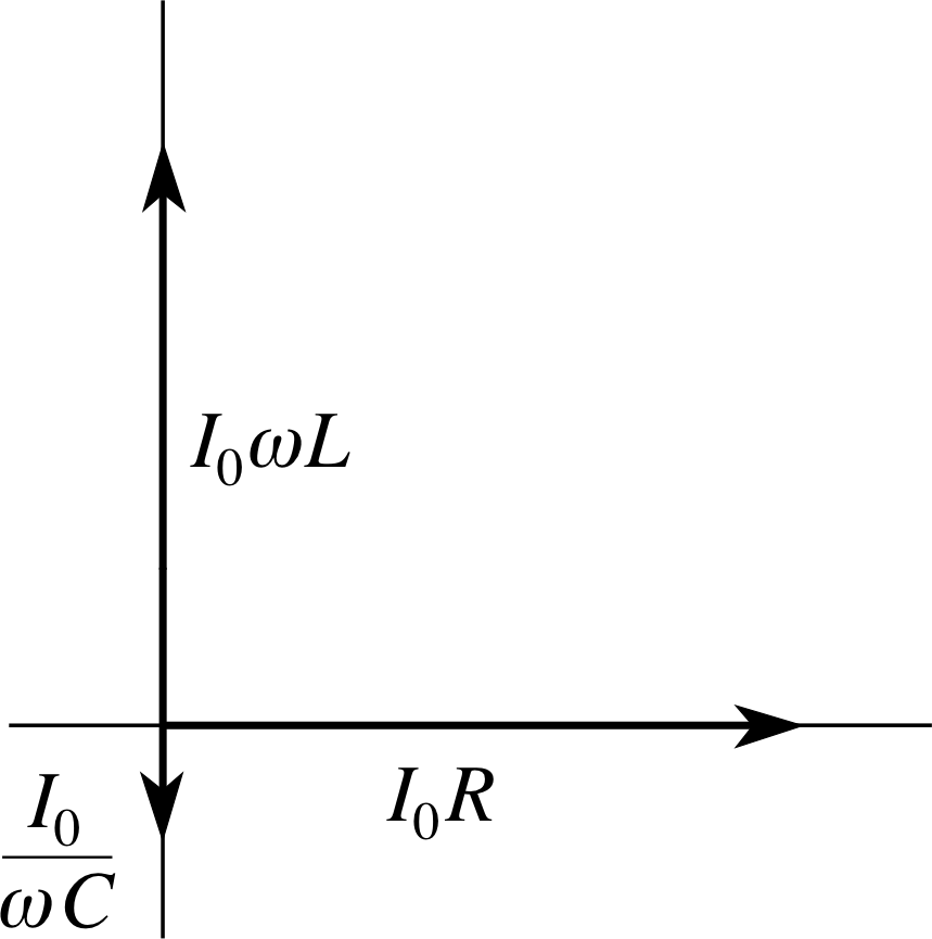
Figure 28 See Answer E3.
The phasor diagram required is shown in Figure 28. The whole diagram may be rotated through an arbitrary angle.
The impedance of a series LCR circuit is given by $Z = \sqrt{\smash[b]{R^2 + (X_C - X_L)^2}}$. Using the same equations as in Answer E2, XL can be calculated as 47 Ω and XC as
8 Ω.
Therefore$Z = \sqrt{50^2 + 39^2}\,\Omega = 63\,\Omega$
The rms current is given by
Irms = Vrms /Z = 80 V/63 Ω = 1.26 A
The current is the same through each component since they are connected in series.
(If you had difficulty with this question, reread Subsections 2.4, 2.5 and 2.6.)
Question E4
(A3 and A6) Describe the energy changes which take place when charge flows in a series a.c. circuit which contains only a capacitor and an inductor. If a resistor is now added to the circuit, what effect will this have on the energy changes?
Answer E4
In a series LC circuit, no energy is lost from the system. Energy ebbs and flows between the electric field in the capacitor and the magnetic field in the inductor, as charge oscillates around the circuit.
When the circuit contains a resistive element, electrical energy is dissipated as heat, and the electrical energy within the circuit decreases with time.
(If you had difficulty with this question, reread Subsections 3.1, 3.2, 3.3 and 3.4.)
Question E5
(A7) Starting from an appropriate condition concerning the total voltage drop around a circuit, show that the stored charge q (t) in a series LCR circuit that contains no external supply must satisfy an equation of the form:
$L\dfrac{d^2q}{dt^2} + R\dfrac{dq}{dt} + \dfrac{q(t)}{C} = 0$
Describe the behaviour of the general solution to this equation in situations where the resistance R is small compared with $\sqrt{4L/C\os}$.
Answer E5
Figure 13 A series LCR a.c. circuit with the relevant phasor diagram showing how the individual voltages are combined. (In this case XC > XL).
Following the sign conventions indicated in Figure 13, we find that the appropriate condition on the voltage drops is
VC(t) + VR(t) + VL(t) = 0
But$V_C(t) = \dfrac{q(t)}{C}$;
$V_R(t) = I(t)R = R\dfrac{dq}{dt}$;
and$V_L(t) = L\dfrac{dI}{dt} = L\dfrac{d^2q}{dt^2}$
where q (t) represents the charge on the top capacitor plate towards which positive conventional currents flow.
So,
$L\dfrac{d^2q}{dt^2} + R\dfrac{dq}{dt} + \dfrac{q(t)}{C} = 0$
If R is small compared with $\sqrt{4L/C\os}$, the solutions to this equation describe (underdamped) oscillations with an amplitude that decays exponentially with time. The angular frequency of the oscillations is given by
$\omega = \sqrt{\dfrac{1}{LC}-\dfrac{R^2}{4L^2}}$
(If you had difficulty with this question, reread Subsection 3.4.)
Question E6
(A7) For the circuit discussed in Question E5, sketch graphs showing the variation with time of the voltage across the capacitor for undamped and overdamped oscillations. State what conditions must be obeyed in each of these cases, and comment on the angular frequency of any oscillations that arise.
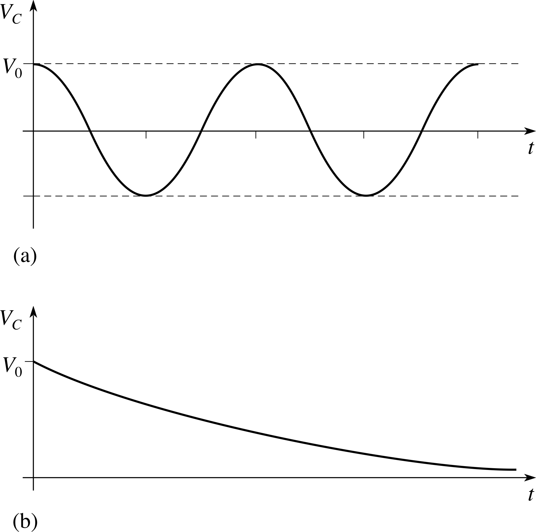
Figure 29 See Answer E6.
Answer E6
The voltage across the capacitor is given by VC(t) = q (t)/C, and we know from Question E5 that q (t) exhibits damped oscillations. Graphs showing the variation of capacitor voltage against time for undamped (Figure 29a), and overdamped oscillations (Figure 29b) in a series LCR circuit are shown in Figure 29.
For undamped oscillations the circuit must have R = 0. The oscillation frequency is then given by $\omega_0 = \sqrt{1/(LC)\os}$. This is larger than $\sqrt{4L/C\os}$ and there is no oscillation as such.
(If you had difficulty with this question, reread Subsections 3.3 and 3.4.)
Question E7
(A8) Under what conditions will the current in an LCR circuit display resonance? Sketch a graph showing this effect and indicate the effect of increasing or decreasing the resistance in the circuit.
Answer E7
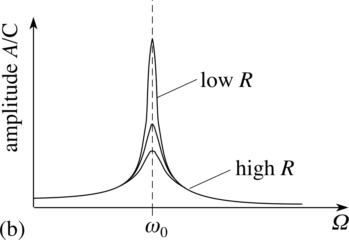
Figure 25b See Answer E6.
A series LCR circuit will display resonance if it is driven by an external voltage supply with an angular frequency Ω that is close to the natural angular frequency $\omega_0 = \sqrt{1/(LC)\os}$ of the circuit in the absence of driving or damping. Under these conditions
XL = XC and $Z = \sqrt{\smash[b]{R^2 + (X_C - X_L)^2}} = R$
At resonance the stored charge will be described by an expression of the form:
$q(t) = A\sin({\it\Omega}t + \phi)$
so$I(t) = \dfrac{q(t)}{dt} = A{\it\Omega}\cos({\it\Omega}t + \phi)$
whereA and ϕ are constants whose values depend on Ω. The variation of A with Ω is shown in Figure 25b.
(If you had difficulty with this question, reread Subsection 3.5.)
Figure 25b A graph showing the variation of the amplitude of the oscillations with Ω.
Study comment This is the final Exit test question. When you have completed the Exit test go back and try the Subsection 1.2Fast track questions if you have not already done so.
If you have completed both the Fast track questions and the Exit test, then you have finished the module and may leave it here.
Study comment Having seen the Fast track questions you may feel that it would be wiser to follow the normal route through the module and to proceed directly to the following Ready to study? Subsection.
Alternatively, you may still be sufficiently comfortable with the material covered by the module to proceed directly to the Section 4Closing items.