PHYS 3.3: Electric charge, field and potential

4 Electric potential and electric field

4.1 Electrostatic potential energy

4.2 Electric potential: definition and representation

4.3 Millikan’s experiments to measure e

5 Point discharge and thunderstorms

6 Closing items

6.3 Exit test

Data for Fast track questions:

ε₀ = 8.85 × 10⁻¹² C² N⁻¹ m⁻²

e = 1.60 × 10⁻¹⁹ C

A precise definition of the coulomb is given at the end of this subsection.

The nuclear model of the atom dates from the beginning of the 20th century. Its development is discussed elsewhere in FLAP.

Millikan’s experiments are described in Subsection 4.3.

There are theoretical reasons for believing that individual quarks can never be isolated and examined individually. Attempts to isolate particles with charges less than e simply seem to result in the production of yet more particles with charges that are integer multiples of e.

Charge ranks alongside other quantities such as energy and momentum which are also believed to be exactly conserved.

Franklin’s choice of which charge–type to label positive and which negative was entirely arbitrary, however it has an unfortunate consequence when considering electric currents. It is conventional to think of current as a flow of positive charge but currents are usually caused by the movement of electrons which are negative using Franklin’s labelling. This means that conventional currents flow in the opposite direction to the corresponding electron flow – a confusing complication which could have been avoided if Franklin had made a different choice.

An ion is an atom that has lost or gained one or more electrons, thus acquiring a net charge.

There is an important class of materials which behave as conductor_electricalconductors in some circumstances and insulator_electricalinsulators in others. They are known as semiconductors and are of great importance in the electronics industry. See the Glossary for further details.

The electrostatic force, Coulomb’s law and inverse square law forces in general are discussed more fully elsewhere in FLAP.

A charge distribution is said to be spherically symmetric if the charge density at any point depends only on the distance from the centre of the distribution and is independent of direction. In the analogous case of gravitation, the result that a spherically symmetric distribution of mass behaves like a point mass is known as Newton’s theorem; consult this entry in the Glossary for further details.

Note that in this case, where a change of sign would indicate a change of direction, the formula involves q₁q₂ rather than |q₁q₂|.

It is useful to remember that 1/(4πε₀) ~ 10¹⁰ N m² C⁻². More precisely, 1/(4πε₀) ≈ 8.988 × 10⁹ N m² C⁻².

As well as being generated by charges, electric fields are also produced by varying magnetic fields – which is how an electric dynamo works. This is dealt with elsewhere in FLAP.

The word ‘positive’ is not really needed in this statement since reversing the sign of the charge also reverses the direction of the force. However, thinking of the field direction as the direction of the force on a positive charge can reduce the need for mental gymnastics and may make the concept easier to grasp.

An equivalent unit, the volt per metre (V m⁻¹), is more common in practice.

In some texts, the dipole moment is defined as a vector p of magnitude qd pointing from the negative to the positive charge. Here dipole moment is simply taken as the scalar quantity qd.

These are assertions, you are not expected to be able to either derive or remember these general expressions on the basis of this discussion.

The noble, or rare, gases include helium, neon and argon. They are listed in Group 8 of the periodic table of elements, and are sometimes known as inert gases because of their extreme reluctance to form compounds.

Newton’s second law of motion: F = ma.

The work ∆W done when a constant one–dimensional force F_x moves through a displacement ∆x is given by ∆W = F_x∆x.

Note that E_kin represents an amount of energy, but E_x is an electric field component. Do not allow the similarity of the symbols to disguise the radically different nature of these two quantities.

It is possible to introduce a potential energy of this kind because the electrostatic force has the property of being conservative_forceconservative. That is to say, the work done by the electrostatic force when an object moves from one point to another is independent of the path taken. The gravitational force and the electrostatic force are both conservative forces to which the idea of potential energy can be applied.

Mass of an electron is 9.1 × 10⁻³¹ kg.

Remember, E_x(r) is just a scalar quantity, the x–component of the electrostatic field at the point with coordinates (x, y, z). Many authors would simply write it as E_x, but we prefer to include the (r) to remind you that it varies from point to point.

∑ is the summation symbol and represents an instruction to add together all terms of the form that follows between any stated limits. See the Glossary for further details if necessary.

See the Glossary for more information about line integrals and their evaluation.

Equation 12b,

$\displaystyle \Delta E_{\rm el} = -q\int_{r_1}^{r_2} {\boldsymbol E}({\boldsymbol r}){\boldsymbol \cdot}d{\boldsymbol r}$

is a general result.

Equation 10,

∆E_el = −qE_x∆x

may be regarded as the outcome of applying this to the case of a uniform field.

If you are not familiar with the process of integration you should simply accept the result given in Equation 12d,

$\Delta E_{\rm el} = \dfrac{qQ}{4\pi\varepsilon_0}\left(\dfrac{1}{r_{\rm B}}-\dfrac{1}{r_{\rm A}}\right)$

∞ is the symbol for infinity.

This is the outcome of applying Equation 12b,

$\displaystyle \Delta E_{\rm el} = -q\int_{r_1}^{r_2} {\boldsymbol E}({\boldsymbol r}){\boldsymbol \cdot}d{\boldsymbol r}$

to the special case of the field of a point charge, and combining the result with the convention that E_el = 0 when r → ∞.

Electric potential is sometimes given the symbol V_el to distinguish it from gravitational potential V_g. However, where there is no risk of confusion, it is usual simply to use V for electric potential and to refer to it as simply ‘the potential’.

Gravitational potential is discussed elsewhere in FLAP.

The electronvolt has wider applications than just the energies of electrically–accelerated charged particles. For example, the energy associated with the vibration of a molecule, or the energy of gamma_radiationγ–ray photon, could be expressed in eV.

In the general case where the potential depends on x, y and z we may write it as V(r) or V(x, y, z) and the three components of the electric field at any point are given by the partial derivatives

$E_x = -\dfrac{\partial V}{\partial x},\;\; E_y = -\dfrac{\partial V}{\partial y},\;\; E_z = -\dfrac{\partial V}{\partial z}$

For an object mass m the gravitational force is directed downward and has magnitude F = mg, where g is the gravitational field strength (or acceleration due to gravity).

Falling through a viscous medium, such as air, an object will reach a constant (terminal) velocity when the drag force of the medium balances the gravitational force. For a sphere of mass m and radius r falling in a medium of viscosity η, terminal velocity υ is reached when mg = 6πrηυ (η is the Greek letter eta).

X–rays ionize the air, producing free electrons and positive ions which may become attached to an oil droplet and hence alter its charge.

g = 9.81 N kg⁻¹.

The same idea applies in the context of a gravitational field: objects will fall towards the Earth if they are able, thus minimizing their gravitational potential energy.

Remember that field lines are always at 90° to an equipotential line or surface.

Any insulator will undergo electrical breakdown if subjected to a sufficiently strong electric field.

1 Opening items

1.1 Module introduction

It is difficult for us in the technologically developed world to imagine life without electricity. It provides light, heat, the power to run railways and underpins the whole electronics industry. All of these applications depend on electric charges moving in response to an electric field.

Electricity is the source of spectacular natural phenomena such as the aurora borealis and lightning. Lightning is of particular concern to people caught in thunderstorms in exposed places. The Mountain Leadership Guide includes the following advice to avoid being struck by lightning:

Move away from peaks. Do not shelter under trees or boulders. Find a place in the open about the same distance from a peak or projection as its height. Sit with your knees drawn up and your hands in your lap. Do not lean back or support your weight on your hands.

Is this good advice? If so why? Could it be improved on? What causes lightning in the first place? These questions will be discussed in Section 5 of this module but first we will establish the fundamentals of field, charge and potential.

We begin in Section 2 with electric charge and Coulomb’s law, then in Section 3 we apply ideas about electric fields to an electric dipole, and see how van der Waals forces ensure that water is a liquid. In Section 4 we review and summarize some key ideas about electrostatic potential energy, electric potential and equipotentials before moving on to a discussion of point discharge and thunderstorms in Section 5.

Study comment Having read the introduction you may feel that you are already familiar with the material covered by this module and that you do not need to study it. If so, try the following Fast track questions. If not, proceed directly to the Subsection 1.3Ready to study? Subsection.

1.2 Fast track questions

Study comment Can you answer the following Fast track questions? If you answer the questions successfully you need only glance through the module before looking at the Subsection 6.1Module summary and the Subsection 6.2Achievements. If you are sure that you can meet each of these achievements, try the Subsection 6.3Exit test. If you have difficulty with only one or two of the questions you should follow the guidance given in the answers and read the relevant parts of the module. However, if you have difficulty with more than two of the Exit questions you are strongly advised to study the whole module.

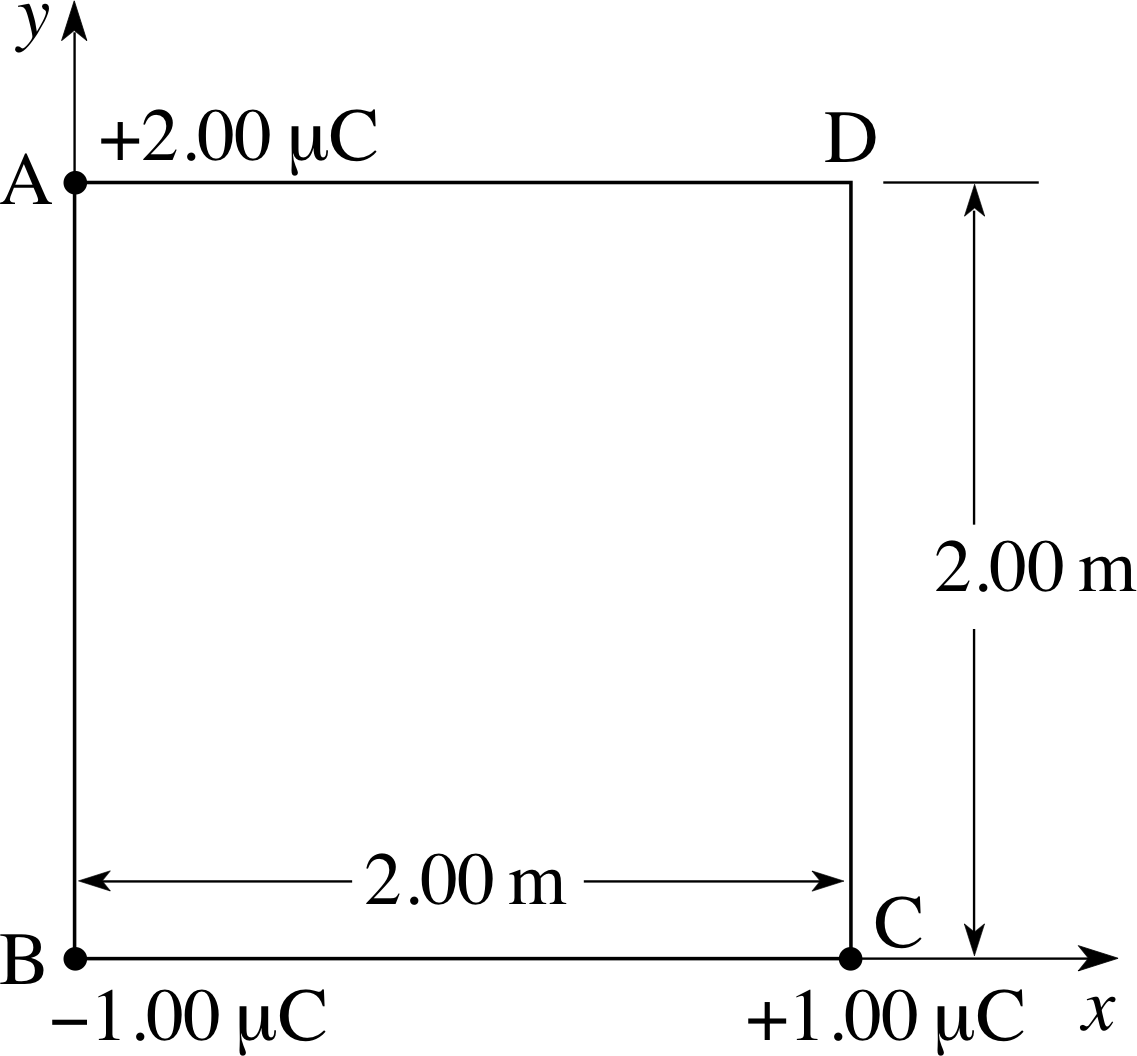
Figure 1 See Question F1.

Question F1

Three charges of +2.00 μC, −1.00 μC and +1.00 μC are positioned at the corners A, B and C of a square as shown in Figure 1. Calculate (a) the x– and y–components of the electric field at point D, (b) the electric potential at D, and (c) the x– and y–components of the force experienced by a charge of −2.00 μC at D.

Answer F1

(a) At point D in Figure 1 the electric field is the sum of the fields due to the charges at A, B and C. By Pythagoras’s theorem, the diagonal of the square is 2.83 m. Using x– and y–directions as indicated in Figure 1 gives us:

E_x = E_xA + E_xB + E_xC and E_y = E_yA + E_yB + E_yC

where E_xA (for example) represents the x component at D of the electric field E_A(r) due to the point charge at A. Using the general expression for the field of a point charge, and making due allowance for the different directions of E_A, E_B and E_C at D we have:

$E_x = \dfrac{Q_{\rm A}}{4\pi\varepsilon_0 r_{\rm AD}^2} = \dfrac{Q_{\rm B}}{4\pi\varepsilon_0 r_{\rm BD}^2}\cos 45° + 0$

i.e.$E_x = \rm \left(\dfrac{+2.00\times 10^{-6}}{4\pi\times 8.85\times 10^{-12}\times 2.00^2} + \dfrac{-1.00\times 10^{-6}\cos 45°}{4\pi\times 8.85\times 10^{-12}\times 2.83^2}\right)\,V\,m^{-1}$

soE_x = 3.70 × 10³ V m⁻¹

Similarly,$E_y = \dfrac{Q_{\rm C}}{4\pi\varepsilon_0 r_{\rm CD}^2} = \dfrac{Q_{\rm B}}{4\pi\varepsilon_0 r_{\rm BD}^2}\sin 45° + 0$

i.e.$E_y = \rm \left(\dfrac{-1.00\times 10^{-6}\sin 45°}{4\pi\times 8.85\times 10^{-12}\times 2.83^2} +\dfrac{+1.00\times 10^{-6}}{4\pi\times 8.85\times 10^{-12}\times 2.00^2}\right)\,V\,m^{-1}$

soE_y = 1.45 × 10³ V m⁻¹

(b) The potential at D is the sum of the potentials due to the charges at A, B and C

V = V_A + V_B + V_C

Using V = Q/4πε₀r

$V = \dfrac{Q_{\rm A}}{4\pi\varepsilon_0 r_{\rm AD}} + \dfrac{Q_{\rm B}}{4\pi\varepsilon_0 r_{\rm BD}} + \dfrac{Q_{\rm C}}{4\pi\varepsilon_0 r_{\rm CD}}$

i.e.$V = 8.99\times 10^3\left(\dfrac{2.00}{2.00} - \dfrac{1.00}{2.83} + \dfrac{1.00}{2.00}\right)\,{\rm V}$

soV = 1.03 × 10⁴ V

F_x = −2.00 × 10⁻⁶C × 3.70 × 10³ N C⁻¹ = −7.40 × 10⁻³ N

andF_y = −2.00 × 10⁻⁶C ×1.45× 10³ N C⁻¹ = −2.90 × 10⁻³ N

Question F2

(a) Calculate the electric dipole moment of an electron and proton separated by 1.2 × 10⁻¹⁰ m.

(b) At a certain point 1.0 × 10⁻⁸ m from the dipole, the electric field has magnitude 5.0 × 10⁵ N C⁻¹. What would be the magnitude of the field at a distance of 1.0 × 10⁻⁷ m from the dipole in the same direction?

Answer F2

(a) Dipole moment = magnitude of charge × separation

i.e.p = 1.6 × 10⁻¹⁹ C × 1.2 × 10⁻¹⁰ m = 1.9 × 10⁻²⁹ C m

(b) At distances large compared to the separation of charges, the field strength due to a dipole falls off as 1/r³. If r is increased by a factor 10, the field strength is reduced by a factor 10³, i.e. to 5.0 × 10² N C⁻¹.

Question F3

(a) What is the distinction between the electrostatic potential energy of a charge q at some point r in an electric field E(r) and the electric potential at the same point?

(b) The potential of a certain distribution of charges depends only on the distance r from a fixed reference point. If the potential is given by V(r) = −ar, where a is a positive constant, what will be the force on a point charge of 2.00 × 10⁻⁶ C at a distance of 4.00 m from the reference point?

Answer F3

(a) The electric potential at any point is the electrostatic potential energy per unit charge at that point.

(b) In this case the equipotential surfaces will be concentric spheres, centred on the reference point. The electric field will be at right angles to the equipotentials, so its only non–zero component will be the radial one given by

$E_r(r) = -\dfrac{dV}{dr}$

Since the relationship between V and r is described by a straight line of gradient −a, it follows that in this case E_r(r) = −(−a) = a. Since a is positive, the field is directed away from the reference point. The force on a charge q due to this field will be given by F_r = qE_r(r), so in this case F_r = (2.00 × 10⁻⁶ C) × a. This force does not depend on the distance from the reference point (so the 4.00 m is irrelevant) and is directed away from the reference point.

Study comment Having seen the Fast track questions you may feel that it would be wiser to follow the normal route through the module and to proceed directly to the following Ready to study? Subsection.

Alternatively, you may still be sufficiently comfortable with the material covered by the module to proceed directly to the Section 6Closing items.

1.3 Ready to study?

Study comment In order to study this module you will need to be familiar with the following terms: atom, Cartesian coordinates, displacement, force, kinetic energy, nucleus, potential energy, work and be able to apply the conservation_of_mechanical_energyprinciple of conservation of energy. Vectors are used extensively in this module: you must be familiar with the use of components_of_a_vectorcomponents and with the procedure for adding vectors (vector addition) and multiplying them by scalars (scaling_of_a_vectorscaling). It would also be useful (though not essential) to have met the notions of scalar product before. You should also be familiar with the basic ideas of calculus, including the use of derivatives to represent gradients of graphs, and definite integrals to represent certain sums. However, you will not be required to evaluate integrals for yourself, so you do not need to be familiar with the techniques for doing so. Several of these terms are reviewed briefly in the course of this module but unless you are already fairly familiar with them you should consult the FLAP modules where they are discussed more fully. You can review them now by referring to the Glossary which will indicate where in FLAP they are developed. The following questions will allow you to establish whether or not you need to review some of these topics before embarking on this module.

Question R1

Two vectors A and B lie in the (x, y) plane. The magnitude_of_a_vector_or_vector_quantitymagnitude of A is A = |A| = 2, and A makes an angle of 30° with the positive x–axis. B = |B| = 4 and B makes an angle of 30° with the positive y–axis (both angles are measured clockwise from the axis mentioned). Calculate the x– and y–components_of_a_vectorcomponents of C and D where C = A + B and D = A − B.

Answer R1

Resolving A and B into x and y components:

A_x = 2cos30° = 1.732, A_y = −2sin30° = −1.000

B_x = 4sin30° = 2.000, B_y = 4cos30° = 3.464

SoC_x = A_x + B_x = +3.732

C_y = A_y + B_y = +2.464

D_x = A_x − B_x = −0.268

D_y = A_y − B_y = −4.464

Consult vectors and components_of_a_vectorcomponents in the Glossary for further information.

Question R2

An archer (unwisely) fires an arrow vertically upwards. If the mass of the arrow is 25 g and the bow gives it an initial kinetic energy of 60 J, what is the potential energy of the arrow when it reaches its maximum height? What will be its speed on returning to the point from which it was fired?

(You can assume air resistance is negligible.)

Answer R2

The kinetic energy is given by E_kin = mυ²/2 = 60 J. Ignoring air resistance, the sum of the kinetic energy and the potential energy will be constant in accordance with the principle of conservation of energy. So at maximum height all the kinetic energy is converted into potential energy E_pot

thusE_pot = 60 J

On returning to the starting point, all the total energy is entirely reconverted into kinetic energy

So$\upsilon = \sqrt{\dfrac{2E_{\rm kin}\os}{m}} = \rm \sqrt{\dfrac{120\os}{0.025}}\,m\,s^{-1} = 69.3\,m\,s^{-1}$

Consult conservation_of_mechanical_energyprinciple of conservation of energy in the Glossary for further information.

2 Electric charge

2.1 A brief history of electric charge

At some time in your life you must have rubbed a balloon on a woollen pullover and then stuck it to the wall or ceiling (if you haven’t, we suggest you try it at the first available opportunity). When you do this you are observing directly the force between electric charges. Similar observations were made by the ancient Greeks, who noticed that rubbing a piece of amber endowed it with strange properties including the ability to attract small particles. Indeed the word ‘electricity’ derives from the Greek elektron meaning amber.

Later experiments, especially in the 18th century, established that many materials exhibit such properties and that there are ‘two kinds of electricity’. Objects with the same kind repel each other; objects with different kinds attract each other. The ‘two kinds of electricity’ can also neutralize each other if brought together and for this reason the pioneering scientist Benjamin Franklin (1706–1790) labelled them positive and negative. The quantity of either kind of electricity in a body is now known as the electric charge of the body and may be expressed as a multiple of the SI unit of charge, the coulomb (C). i

Electrically charged particles play a fundamental part in nature; all the familiar forms of matter are ultimately composed of them. The atoms that make up gases, liquids and solids consist of negatively–charged particles called electrons swarming around a central nucleus that contains positively–charged particles called protons and uncharged neutrons. i Although the charges of protons and electrons differ in sign they both have the same magnitude, usually denoted by the (positive) quantity e. In 1909, the American physicist Robert Millikan (1868–1953) began a series of experiments with electrons which indicated that the magnitude of the charge on the electron is e ≈ 1.6 × 10⁻¹⁹ C. i Numerous experiments since then have confirmed this result and the most accurate value to date is

e = (1.602 177 38 ± 0.000 000 48) × 10⁻¹⁹ C

At the present time, every charged particle that has been experimentally isolated has been found to have a charge that is equal to e multiplied by some positive or negative whole number. This phenomenon is often described as the quantization of charge since it indicates that e is a fundamental ‘unit’ or ‘quantum’ of charge. The origin of charge quantization is still not fully understood, and there is strong evidence that various particles, including protons and neutrons, contain constituents called quarks, with charges 2e/3 and −e/3. However, it does not appear to be possible to isolate individual quarks, so the directly observable fundamental charge remains e rather than e/3. i

Under normal circumstances, a sample of ordinary matter contains the same number of protons and electrons so that the effects of their charges cancel exactly and most objects are electrically neutral. Yet it is worth reflecting that the amount of charge contained in macroscopic objects is enormous. Your body contains something like 10²⁸ protons and electrons, equivalent to 10⁹ C of each kind of charge.

Another observed property of electric charge is that the net quantity of electric charge in the universe never changes. Charged particles can be created or destroyed in nuclear and subnuclear processes, but whenever this happens it always involves groups of two or more particles and occurs in such a way that the net charge at the start of the process is equal to the net charge at the end of the process. This observation is embodied in the principle of conservation of charge:

The net amount of charge in the universe is constant. i

Defining the coulomb

This module is concerned primarily with electrostatics – the study of situations in which electric charges are stationary, or as near stationary as to make no difference. However, the formal definition of the coulomb, the SI unit of charge, is based on the concept of an electric current which involves the movement of charge. The SI unit of electric current is the ampere which may defined as follows:

The ampere (A) is that constant current which, if maintained in each of two infinitely long, straight, parallel wires of negligible cross section, placed 1 metre apart, in a vacuum, will cause each wire to experience a force of magnitude 2 × 10⁻⁷ N per metre of its length.

Now, if a constant current flowing in a wire causes a quantity of charge ∆q i to flow past a fixed point in time ∆t, we say that the current in the wire (expressed in amperes, or amps for short) is

$I = \dfrac{\Delta q}{\Delta t}$

It follows from this that we may define the coulomb as follows:

1 coulomb is the amount of charge transferred when an electric current of 1 ampere flows for 1 second, so 1 C = 1 A s.

✦ It was mentioned earlier that your body contains about 10⁹ C of each kind of charge. How long would it take for a current of 1.00 A flowing past a fixed point on your body to transfer 1.00 × 10⁹ C?

✧ ∆t = ∆q/I = (1.00 × 10⁹ C)/(1.00 A) = 1.00 × 10⁹ s ≈ 31.7 years.

2.2 Charging by contact and by induction

When two suitable materials (for example glass and silk, or polythene and wool) are rubbed together, one acquires a net positive charge and the other a net negative charge. The exact mechanism is not completely understood but it is clear that electrons or ions must have been transferred between the two materials. If the materials were originally electrically neutral, they will acquire equal and opposite net charges as a result of the charge transfer. i These net charges will each be an extremely tiny fraction (perhaps 1/10¹⁵) of the total positive and negative charges available within the two objects.

Materials can be broadly classified according to the freedom with which charge can move within them. An electrical conductor is a material in which charge moves freely; examples include metals, bodily fluids and tap water. Metals are good conductors because they contain many electrons which are only weakly held to individual atoms. In other materials such as salt solution or bodily fluids, it is ions rather than electrons which are free to move. A material in which charge does not move freely is called an electrical insulator. Dry wood, rubber and most plastics are examples of insulators. i Excess charge deposited on an insulator tends to remain localized near the point of deposition.

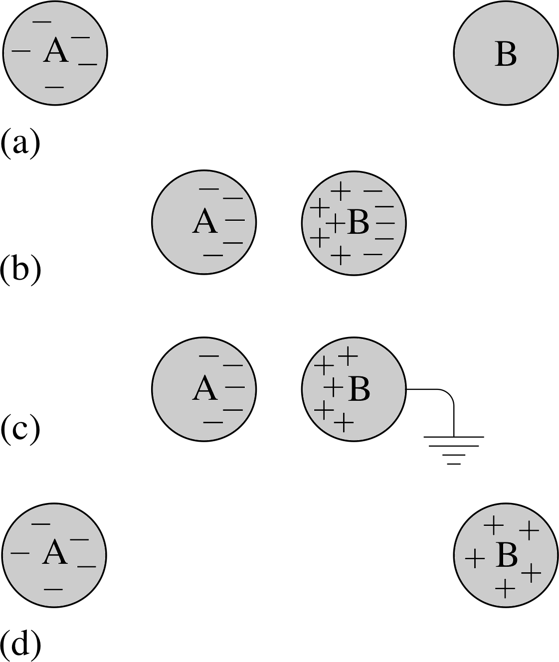
Figure 2 Charging by induction. (a) A negatively charged body (A) and a neutral conductor (B). (b) The conductor is brought close to the charged body giving rise to some separation of positive and negative charge. (c) The side furthest from the charged body is connected to the Earth (as indicated by the special earth symbol) and the excess negative charge migrates along this connection. (d) The conductor is now positively charged. The charged body retains its original negative charge.

If a conductor carries a net charge, positive or negative, the mutual repulsion between like charges will tend to force the excess charges to the surface of the conductor. Consequently, given the highly mobile nature of charges in a conductor, we never expect to find any net static charge inside an isolated conductor. This also ensures that there is no net electrical force within the conductor. If a conductor is brought near to a charged object, the charges within the conductor will redistribute themselves in such a way that the net force on each charge is zero. This redistribution of charge again ensures that there are no net electrical forces anywhere inside a conductor – and this applies to the space inside a hollow conductor as well as to a solid conducting body.

This useful result is exploited in electrostatic screening: if you want to protect something (such as a delicate piece of apparatus) from any external electrical influences, you simply enclose it in a metal container.

If a charged conductor is brought into contact with an uncharged conductor, the excess charge will be distributed between the two; this charge sharing means that the second conductor becomes charged. Once again the redistribution will eliminate net electrical forces within the conductor.

Charge can also be accumulated on conductors by a process known as electrostatic induction. If, say, a negatively charged body is brought close to a conductor, negative charges on the conductor will be repelled and positive charges will be attracted. The net effect will be a separation of charge on the conductor. If the side opposite the charged body is now connected to the Earth (which can be regarded as a huge conductor), negative charge will flow to the Earth leaving the conductor with an overall positive charge. This process is illustrated in Figure 2.

Note The term induction is also used to describe the production of electric current from a changing magnetic field. This is a completely unrelated use of the word. In this module induction will always mean electrostatic induction.

✦ Figure 2 illustrates the fact that when a charged body is connected to the Earth, free excess charge will flow from the body to the Earth. Why does this happen?

✧ The Earth can be regarded as a huge neutral conductor. When connected to a smaller, charged conductor, the excess charges redistribute themselves over both bodies until all the electric forces balance. Because the Earth is so enormous, virtually all the excess charge flows to it.

This process of earthing is very useful in many areas of electricity.

When a body is connected to the Earth by a conducting pathway we say it is earthed, or connected to earth. The process of connecting a body to earth is called earthing.

2.3 Coulomb’s law and electrostatic forces

The nature of the force between charges was first investigated by Charles Augustin de Coulomb (1736–1806) in 1785. In a series of painstaking experiments he looked at the way in which the force between charged bodies varies with their separation and with the size and sign of the charge. His work resulted in Coulomb’s law which can be stated as follows: i

The magnitude of the electric force between two charged particles is proportional to the product of their charges and inversely proportional to the square of the distance between them. The force is directed along a line joining the particles and is repulsive for charges of the same sign and attractive for charges of opposite sign.

The force between charged particles is referred to as the Coulomb force or the electrostatic force. i

Coulomb’s law is expressed in terms of charged particles (that is charges whose dimensions are vanishingly small). However, a spherically symmetric charge distribution of total charge q has exactly the same effect at any point beyond its own surface as a point charge q located at the geometric centre of the distribution. i Thus, any results that are derived for point charges will also apply to spherically symmetric charge distributions, such as charged spheres, provided we confine our attention to points that are outside the distribution concerned.

In mathematical terms, Coulomb’s law implies that the magnitude of the electrostatic force on a point charge q₂ due to another point charge q₁ a distance r away is

$F_{\rm el} = [\text{positive constant}] \times \dfrac{\left\lvert\,q_1 q_2\,\right|}{r^2}$(1a)

Because of the 1/r² dependence, we say that the Coulomb force satisfies an inverse square law. Note that F_el is a magnitude, and therefore a positive quantity, that is why Equation 1a involves the modulus |q₁q₂| which is positive, rather than simply q₁q₂which might be positive or negative. Of course, to describe the Coulomb force fully, we need to specify its direction as well as its magnitude. We can do this by introducing a vector r that points from q₁ to q₂ and using it to define a unit vector r^{^}/|r|. Defined in this way, by dividing the vector r by its own magnitude r, the unit vector points in the same direction as r (i.e. from q₁ to q₂) but it has magnitude 1 and is therefore dimensionless and unitless. Using the unit vector we can write the electrostatic force on q₂ due to q₁ as

${\boldsymbol F}_{21} = [\text{positive~constant}] \times \dfrac{q_1 q_2}{r^2}\hat{\boldsymbol r}$(1b) i

If q₁ and q₂ have the same sign q₁q₂ will be positive and the force on q₂ due to q₁ will point in the same direction as r^{^}/|r|, i.e. away from q₁. However, if q₁ and q₂ have opposite signs q₁q₂ will be negative and F₂₁ will point towards q₁.

In the SI system, the positive constant is written as 1/(4πε), where ε is known as the permittivity of the medium between the charges, so

${\boldsymbol F}_{21} = \dfrac{q_1 q_2}{4\pi\varepsilon r^2}\hat{\boldsymbol r}$(1c)

The seemingly unnecessarily complicated form of the constant actually makes calculations easier (honestly!). The factor of 4π often cancels with other factors of 4π which appear because of the spherical symmetry of Coulomb’s law. For charges in a vacuum, ε has the (approximate) value 8.85 × 10⁻¹² C² N⁻¹ m⁻². This is known as the permittivity of free space and is written ε₀. The presence of a medium reduces the force by a factor 1/ε_r, where ε_r (a dimensionless number, greater than 1) is the called relative permittivity of the medium and is defined by

ε = ε₀ε_r

Air has a relative permittivity of ε_r = 1.005, so ε = 8.898 × 10⁻¹² C² N⁻¹ m⁻² for air.

Coulomb forces, like all other forces, are vectors and therefore they can be added according to the normal rules of vector addition. To find the force on a particular charged body due to a number of other charged bodies, we simply add the individual Coulomb forces vectorially.

Question T1

A hydrogen atom consists of 1 electron and 1 proton arranged such that the proton can be considered to be at the centre of a sphere with the electron at a distance of 5.0 × 10⁻¹¹ m away. What is the magnitude of the Coulomb force between them? You may assume that the relevant value of the permittivity is ε₀ in this case. i

Answer T1

Using Equation 1c,

${\boldsymbol F}_{21} = \dfrac{q_1 q_2}{4\pi\varepsilon r^2}\hat{\boldsymbol r}$(Eqn 1c)

and4πε₀ ≈ 1.1 × 10⁻¹⁰ C² N⁻¹ m⁻²

$\lvert\,{\boldsymbol F}\,\rvert = \rm \dfrac{\left(1.6\times 10^{-19}\right)^2}{1.1\times 10^{-10}\times\left(5.0\times10^{-11}\right)^2}\,N = 9.3 \times 10^{-8}\,N$

Question T2

What is the magnitude of the force of attraction between the protons in your body and the electrons in the body of a friend standing 1 km away from you? Why don’t you hurtle towards each other?

Answer T2

Using the figure of ~10⁹ C for the charge in your body quoted in Subsection 2.1

$\lvert\,{\boldsymbol F}\,\rvert = \rm \dfrac{\left(1\times 10^9\right)^2}{1.1\times 10^{-10}\times 1\times 10^6}\,N = 9 \times 10^{21}\,N$

This enormous force even at such a large distance does not send you crashing towards each other because all the attractive forces between protons and electrons are balanced by the equally large repulsive forces between the two sets of protons and the two sets of electrons. In other words there is no net charge on either person and so no net force.

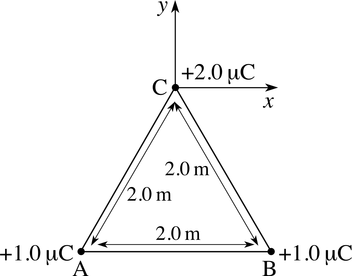
Figure 3 See Question T3.

Question T3

For the arrangement of charges shown in Figure 3, find the force on the charge at C due to the charges at A and B. Recalculate the force if the +1.0 μC charge at A is replaced by a charge of −1.0 μC.

Answer T3

From the symmetry of Figure 3, you should be able to see that the x– components of the two Coulomb forces will cancel leaving only the y– component to worry about. The total y–component is then twice the component from either individual charge. Thus:

$F_y = 2 \times \dfrac{Qq}{4\pi\varepsilon_0 r^2}\cos\theta\quad\text{where}\quad\theta = \dfrac{1}{2}A\hat{C}B = 30°$

so$F_y = \rm \dfrac{2\times 1.0\times 10^{-6}\times2.0\times 10^{-6}\times 0.866}{1.1\times 10^{-10}\times \left(2.0\right)^2}\,N$

i.e.F_y = 7.8 × 10⁻² N

With the charge at A in Figure 3 replaced by −1.0 μC, the resultant force will act in the −x–direction. The magnitude will again be twice that from either individual charge.

so$F_x = \rm \dfrac{-2\times 1.0\times 10^{-6}\times 2.0\times 10^{-6}\times 0.866}{1.1\times 10^{-10}\times \left(2.0\right)^2}\times \cos 60°\,N = -4.5\times 10^{-3}\,N$ (i.e. to the left)

3 Electric fields

3.1 Electric field: definition and representation

Study comment Fields (electric and gravitational) are introduced and discussed more fully elsewhere in FLAP. Consult the Glossary for references to those fuller treatments if you need them.

If you place an electric charge at some distance from another charge or from a group of charges, it experiences an electrostatic force, which acts ‘at a distance’ since there is no material connection between the charges. The question arises: how is the force transmitted? One plausible answer is that the region around a charge has a special property which causes a force to be exerted on other charges within it. This is the attitude conventionally adopted by physicists, and the property concerned is called the electric field.

Thus, rather than thinking of a system of charges genuinely exerting a force ‘at a distance’ on another charge, we prefer to think of a system of charges generating an electric field throughout space and the field acting on any charge placed within it. This may appear to be a rather subtle distinction but this way of thinking has many advantages. In particular, if you can specify the electric field throughout a region in space, you can work out the force on any charge at any point within the region without having to refer back to the system of charges which actually caused the force. i

Having established the general idea that an electric field exists at all points throughout a region of space, we need to know how to quantify it, that is to assign a value to it at every point. Now, the role of the electric field is to tell us the force that would act on a charged particle placed at any point within it, so it makes sense to define the field in terms of that force. The usual procedure is to imagine that we are in possession of a test charge q that is sufficiently small that it will not significantly disturb the field it is being used to measure, and which we can place at any point. If we locate the test charge q at a point with position coordinates (x, y, z) then we can measure the electrostatic force F_el (on q at (x, y, z)) that acts on it at that point. Now you should be able to see from Coulomb’s law that this force will always be proportional to the q itself, so it is not purely characteristic of the charges that produce the electric field. However, if we divide F_el (on q at (x, y, z)) by q then the resulting vector quantity will be independent of q and will be determined by the original charge distribution alone. It is this quantity, F_el (on q at (x, y, z)) divided by q, that defines the electric field at (x, y, z).

Since the electric field is a vector quantity, and since its value varies from point to point, we may symbolize it E(x, y, z), thus we arrive at the basic definition of the electric field:

${\boldsymbol E}(x,\,y,\,z) = \dfrac{{\boldsymbol F}_{\rm el}(\text{on }q\text{ at }(x,\,y,\,z))}{q}$ or F_el = qE(1d)

This is such a fundamental definition that it deserves to be spelt out in words, so that its meaning is absolutely clear.

The electric field at any point is the electrostatic force per unit (positive) charge that would be experienced by a test charge placed at that point. i

Note that the electric field is defined in terms of the force that would be experienced by an appropriately located test charge, so the field exists whether or not a test charge is actually present to experience its effect.

✦ What would be suitable SI units for the measurement of an electric field?

✧ Force may be measured in newtons (N) and charge in coulombs (C). It follows from the general definition given above that the electric field may be measured in units of N C⁻¹. i

It can become rather tedious to repeatedly write E(x, y, z) each time we want to refer to the electric field at a point, so it is common to use the position vector r as a shorthand for the coordinates (x, y, z) and write the field as E(r). We will usually adopt this convention, but it is important to realize that E(r) does not necessarily point in the direction of the position vector r. The role of the parenthetical r is simply to remind you that the magnitude and direction of the electric field will generally vary from place to place. Thus, if we were to write it out in full, in terms of its Cartesian components, we could equally well write the electric field in either of the following forms:

E(r) = (E_x(r), E_y(r), E_z(r))

orE(x, y, z) = (E_x(x, y, z), E_y(x, y, z), E_z(x, y, z))

Many authors avoid such complications entirely by writing the electric field simply as E or (E_x, E_y, E_z) as appropriate, but in doing so they are leaving it to you to remember that the field and its components may vary with position.

Having discussed the general definition of the electric field we can now consider the electric field of a specific charge distribution. The simplest such distribution consists of a single point charge Q at the origin of a Cartesian coordinate system. From Coulomb’s law, the electrostatic force on a test charge q at the point with position vector r = (x, y, z) is then:

${\boldsymbol F} = \dfrac{Qq}{4\pi\varepsilon r^2}\hat{\boldsymbol r}$

where r = |r| = $\sqrt{\smash[b]{x^2 + y^2 + z^2}}$, and r^{^} is the unit vector defined by r^{^} = r/|r|. From this expression for the electrostatic force, and by comparing Equations 1a and 1d

$F_{\rm el} = [\text{positive constant}] \times \dfrac{\left\lvert\,q_1 q_2\,\right|}{r^2}$(Eqn 1a)

${\boldsymbol E}(x,\,y,\,z) = \dfrac{{\boldsymbol F}_{\rm el}(\text{on}~q~\text{at}~(x,\,y,\,z))}{q}$ or F_el = qE(Eqn 1d)

you should be able to see that at any point r the electric field of the point charge Q is:

${\boldsymbol E}({\boldsymbol r}) = \dfrac{Qq}{4\pi\varepsilon r^2}\hat{\boldsymbol r}$(2)

Since the electric field is a vector quantity, the total field at a given position due to a system of point charges can be found using vector addition to add together the electric fields due to each of the charges individually.

Question T4

What is the electric field at a distance of 1.00 m from a point charge of +1.00 C?

Answer T4

As electric field is a vector, Equation 2,

${\boldsymbol E}({\boldsymbol r}) = \dfrac{Qq}{4\pi\varepsilon r^2}\hat{\boldsymbol r}$(Eqn 2)

the magnitude of the electric field is

$E = \dfrac{1.00\,{\rm C}}{4\pi\varepsilon_0 \times 1.00\,{\rm m^2}} = \rm 8.99\times 10^9\,N\,C^{-1}$

and the direction of the field will be away from the charge.

Figure 3 See Question T5.

Question T5

Calculate the electric field at point C in Figure 3 due to the charges at A and B. (You can ignore the charge at C.)

Answer T5

The calculation is similar to that for Question T3, E_y = 2Qcosθ/(4πε₀r²)

$E_y = \rm \dfrac{2\times 1.0\times 10^{-6}\times 0.866}{1.1 \times 10^{-10}\times \left(2.0\right)^2}\,N\,C^{-1} = 3.95\times 10^3\,N\,C^{-1}$

We can represent an electric field diagramatically using electric field lines. These are directed_line_segmentdirected lines (i.e. lines with arrows on them) that have the following properties:

The lines may begin and end on charges, but are otherwise continuous.
The lines are drawn so that at any point the field is tangential to the lines.
At any point the direction of the lines shows the direction of the field. (Since the field is the force per unit positive test charge, the lines are directed away from positive charges and towards negative charges.)
The density of the lines is proportional to the field strength. (‘Density’ is taken to mean the number of lines per unit area perpendicular to the field direction.)

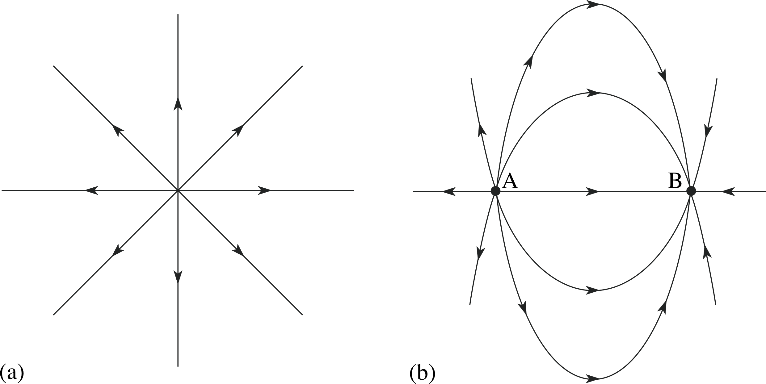
Figure 4 Field lines of (a) an isolated positive charge, (b) two charges of equal magnitude and opposite sign.

Figure 4a shows field lines associated with a (positive) point charge, and Figure 4b shows the field line representation of the electric field surrounding a pair of charges of equal magnitude but opposite sign. Field directions throughout the region of interest, and areas of high and low field strength, can be seen at a glance. Field line diagrams also indicate the relative sizes of charges. If we double the size of the point charge in Figure 4a, we double the field strength everywhere and therefore we need to double the line density everywhere. This means we double the number of lines emanating from the charge.

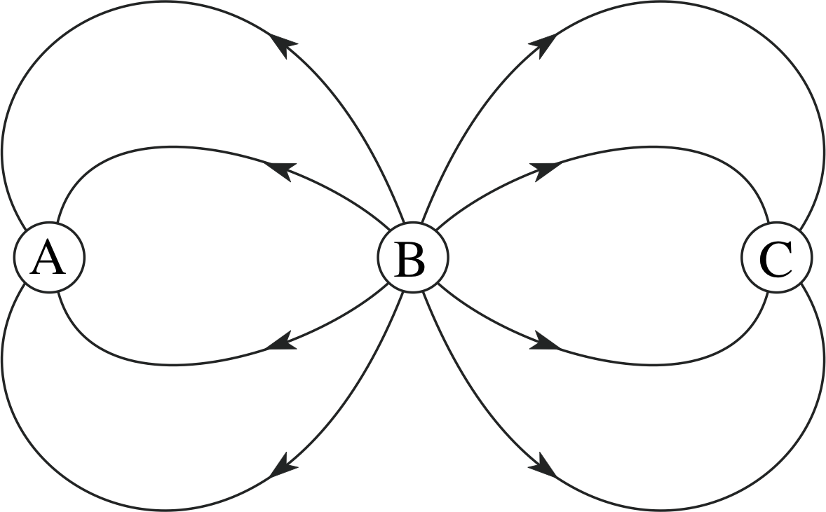
Figure 5 See Question T6.

Question T6

If the positive charge in Figure 5 is +1.0 C, what are the sizes of the other charges in the figure?

Answer T6

The charge magnitudes should be in the same proportions as the number of field lines entering or leaving. The only positive charge is at B since this is the only charge from which field lines radiate, so if q_B = +1 C, q_A = q_C = −0.5 C.

It is worth remarking that the quantitative interpretation of field lines only works because the electric field due to a point charge obeys an inverse square law. It can easily be shown that the density of lines drawn radially from a point also obeys an inverse square law and so is a true representation of the field. As any field can be built up by summing the fields due to a distribution of point charges, so any field can be represented by field lines. If the electric field of a point charge were proportional to 1/r³, say, rather than 1/r², the field line representation would not work.

✦ The electric field at a certain point is given by

E = (E_x, E_y, E_z) = (10 N C⁻¹, 15 N C⁻¹, −20 N C⁻¹)

What is the force F on a particle of charge −4 C located at the point?

✧ It follows from the general definition of the electric field that

F = qE

so in this case

F = (−40 N, −60 N, 80 N)

3.2 The field of an electric dipole

As a further example of the electric field of a distribution of point charges, we will now examine another simple case – the field due to an electric dipole in a vacuum.

An electric dipole consists of two charges of equal magnitude but opposite sign which are very close together.

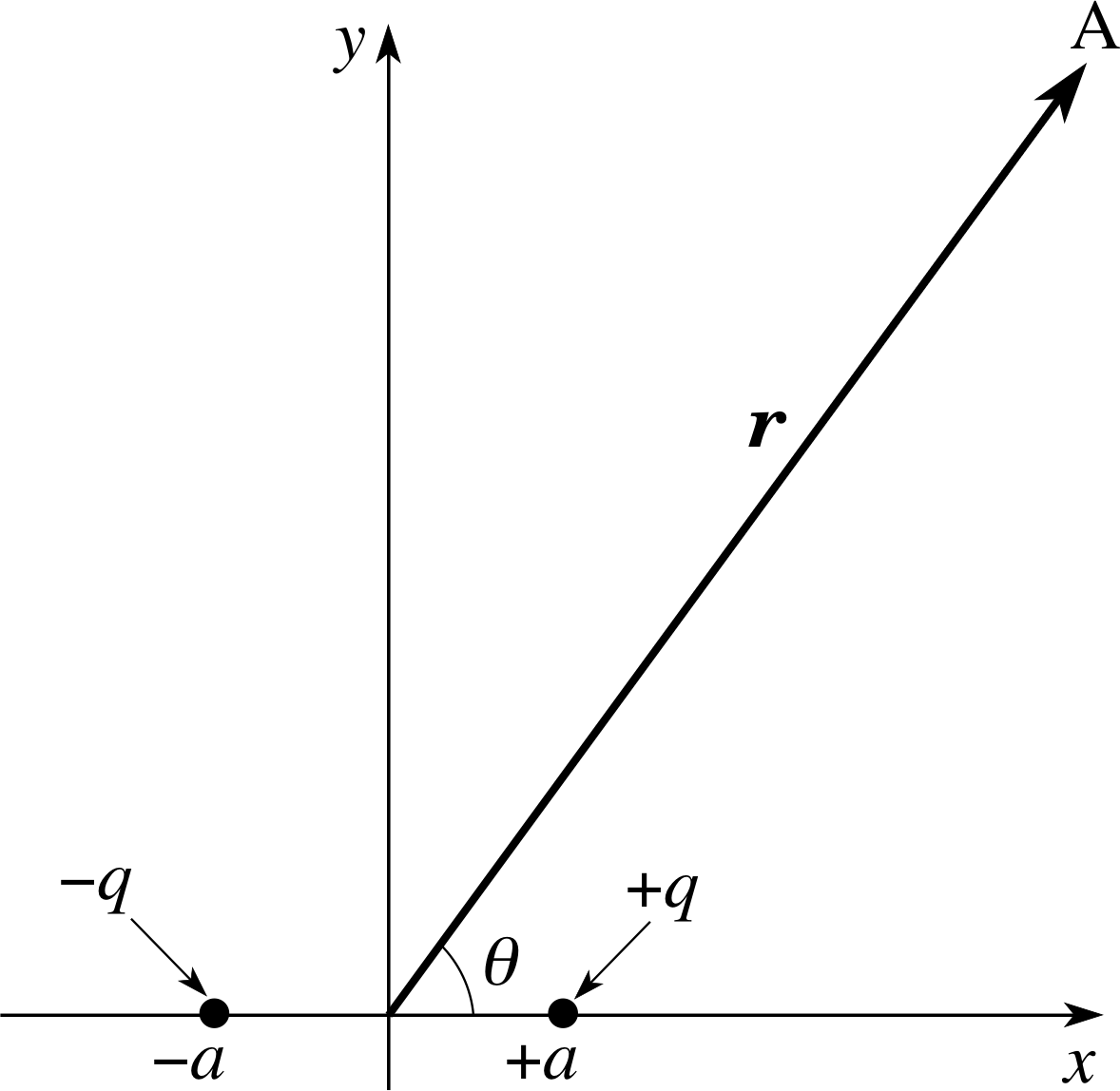
Figure 6 An electric dipole and the position vector r of some arbitrary point A.

Such a pair is shown in Figure 6. For convenience, we choose a coordinate system such that the charges lie on the x–axis, equidistant from the origin, with the charge +q at x = +a and the charge −q at x = −a. Because of the symmetry of this charge distribution we need only consider the field in the (x, y) plane; whatever pattern we find there will be repeated in every other plane that includes the x–axis. We can therefore find the full three–dimensional field pattern by rotating the field in the (x, y) plane about the x–axis. Having effectively reduced the problem to two dimensions we can start by deriving an expression for the field at some point along the x–axis, let us call it (x, 0). As both charges lie on the x–axis, the field vector at (x, 0) will always point in the x–direction, so E_y(x, 0) will be zero and we only need to work out the x–component, E_x(x, 0).

Using subscripts 1 and 2 for the charges at −a and +a, respectively, application of Equation 2,

${\boldsymbol E}({\boldsymbol r}) = \dfrac{Qq}{4\pi\varepsilon r^2}\hat{\boldsymbol r}$(Eqn 2)

in a vacuum where ε = ε₀, gives:

$E_{x1}(x,0) = \dfrac{-q}{4\pi\varepsilon_0 (x+a)^2}$

and$E_{x2}(x,0) = \dfrac{+q}{4\pi\varepsilon_0 (x-a)^2}$

so$E_{x}(x,0) = E_{x1}(x,0) + E_{x2}(x,0) = \dfrac{q}{4\pi\varepsilon_0}\left[\dfrac{1}{(x-a)^2}-\dfrac{1}{(x+a)^2}\right]$

i.e.$E_{x}(x,0) = \dfrac{q}{4\pi\varepsilon_0}\left[\dfrac{(x+a)^2-(x-a)^2}{(x-a)^2(x+a)^2}\right]$

so$E_{x}(x,0) = \dfrac{q}{4\pi\varepsilon_0}\left[\dfrac{4ax}{(x-a)^2(x+a)^2}\right]$

If the charges are very close together, and if we take |x| ≫ a then, to a good approximation

$E_{x}(x,0) = \dfrac{4aqx}{4\pi\varepsilon_0 x^4} = \dfrac{aq}{\pi\varepsilon_0\lvert\,x\,\rvert^3}$(3)

When dealing with the field of a dipole the product of the charge magnitude and separation is called the electric dipole moment p. So, for two charges of magnitude q separated by a distance d:

p = qd(4) i

In this case the separation is 2a, so p = 2aq and Equation 3 may be written

$E_{x}(x,0) = \dfrac{p}{2\pi\varepsilon_0\lvert\,x\,\rvert^3}$(5a)

Recalling that E_y(x, 0) = 0(5b)

we now know the electric field at any point on the x–axis where |x| ≫ a.

Figure 6 An electric dipole and the position vector r of some arbitrary point A.

Question T7

For the dipole in Figure 6, show that at any point on the y–axis with coordinates (0, y), where |y| ≫ a,

$E_x(0,\,y) = \dfrac{-p}{4\pi\varepsilon_0\lvert\,y\,\rvert^3}$(6a)

andE_y(0, y) = 0(6b)

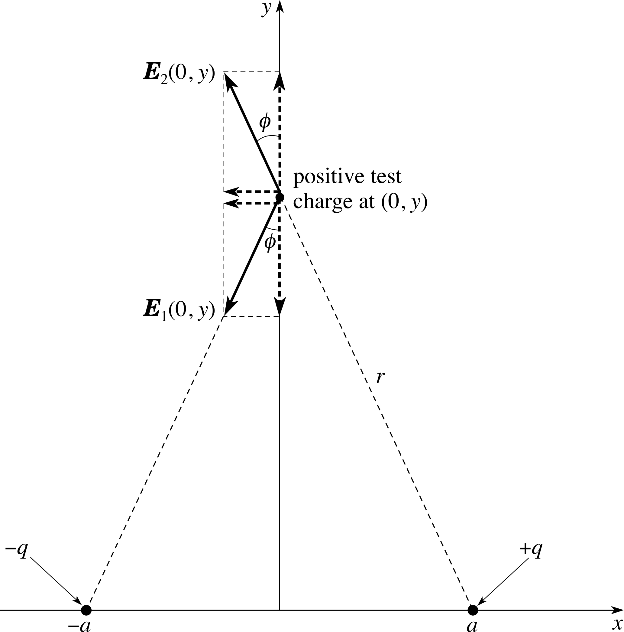
Figure 21 See Answer T7.

Answer T7

See Figure 21. At any point (0, y) the y–components of the fields from the two (oppositely charged) charges will be equal and opposite, so E_y(0, y) = E_y1(0, y) + E_y2(0, y) = 0. Turning to the x–component:

$E_x(0,\,y) = E_{x1}(0,\,y) + E_{x2}(0,\,y) = \dfrac{-q\sin(\phi)}{4\pi\varepsilon_0 r^2} + \dfrac{-q\sin(\phi)}{4\pi\varepsilon_0 r^2}$

wherer² = y² + a² and sinϕ = a/r.

Thus $E_x(0,\,y) = \dfrac{-2q}{4\pi\varepsilon_0 r^2}\times \dfrac{a}{r} = \dfrac{-p}{4\pi\varepsilon_0 r^3}$

but r ≈ |y|, and the approximation becomes increasingly accurate as |y| becomes larger and larger compared with a.

Hence, for |y| ≫ a, $E_x(0,\,y) = \dfrac{-p}{4\pi\varepsilon_0 \lvert\,y\,\rvert^3}$

The derivation of the dipole field on the x– and y–axes (Equations 5 and 6) is relatively straightforward because of the symmetry of the charges. However, it is not so much more difficult (just a bit more long-winded) to derive a general expression for E(x, y) = (E_x(x, y), E_y(x, y)) at any point in the (x, y) plane such as A in Figure 6, provided $r = \sqrt{\smash[b]{x^2+y^2}}\gg a$.

The final result is:

$E_x(x,\,y) = \dfrac{p}{4\pi\varepsilon_0 r^3}(\cos^2\theta - \sin^2\theta)$(7a) i

$E_y(x,\,y) = \dfrac{p}{4\pi\varepsilon_0 r^3}(3\cos\theta \sin\theta)$(7b) i

where r = (x, y) and θ are as shown in Figure 6.

Equations 7a and 7b show that:

At distances r which are large compared with the charge separation, the electric field of a dipole decreases in proportion to 1/r³ and also depends on θ.

Although we now have a complete description of the field in the (x, y) plane, it is still quite difficult to visualize the field. This is where field lines are useful. In fact you have already seen the dipole field in Figure 4b. Figure 4b gives us a ‘feel’ for the way the field behaves. Equations 7a and 7b allow us to do quantitative calculations for the field at any point in space.

Question T8

Show that Equations 7a and 7b

$E_x(x,\,y) = \dfrac{p}{4\pi\varepsilon_0 r^3}(\cos^2\theta - \sin^2\theta)$(Eqn 7a)

$E_y(x,\,y) = \dfrac{p}{4\pi\varepsilon_0 r^3}(3\cos\theta \sin\theta)$(Eqn 7b)

are consistent with Equations 5 and 6,

$E_{x}(x,\,0) = \dfrac{p}{2\pi\varepsilon_0\lvert\,x\,\rvert^3}$(Eqn 5a)

E_y(x, 0) = 0(Eqn 5b)

$E_x(0,\,y) = \dfrac{-p}{4\pi\varepsilon_0\lvert\,y\,\rvert^3}$(Eqn 6a)

E_y(0, y) = 0(Eqn 6b)

Answer T8

For a point on the x–axis in Figure 6, θ = 0 and r ≈ x provided |x| ≫ a. It follows from Equation 7,

that$E_x(x,\,y) = \dfrac{p}{4\pi\varepsilon_0 \lvert\,x\,\rvert^3}\times (2-0) = \dfrac{p}{2\pi\varepsilon_0 \lvert\,x\,\rvert^3}$

andE_y(x, 0) = 0

which agrees with Equation 5 for |x| ≫ a.

For a point on the y–axis in Figure 6, θ = 90° and r ≈ |y| provided |y| ≫ a. It follows from Equation 7,

that$E_y(x,\,y) = \dfrac{p}{4\pi\varepsilon_0 \lvert\,y\,\rvert^3}\times (2\times 0-1) = -\dfrac{p}{2\pi\varepsilon_0 \lvert\,y\,\rvert^3}$

andE_y(0, y) = 0

which agrees with Equation 6 for |y| ≫ a.

3.3 The van der Waals force

There are many situations in the real world which can be approximated by electric dipoles. You have come across one already in Subsection 2.2 in the (a) description of charging by induction. The displaced positive and negative charges on the conductor in Figure 2 behave to a good approximation like two point charges separated by a small distance – an electric dipole.

Many molecules exhibit dipolar behaviour due to asymmetries in the distribution of their electrons. Water is a good example of this. The arrangement of atoms in a water molecule is shown in Figure 7. Electrons spend more time on average near the oxygen atom (O) than near the hydrogen atoms (H) that are bound to it, so the O side of the molecule has a net negative charge while the H side has a net positive charge. In effect it is a dipole.

The mutual attraction between charges of opposite sign on different molecules causes them to clump together (provided their kinetic energy is not too high) eventually forming crystals of solid H₂O or ice. It is this electrostatic attraction between molecular dipoles that allows water to be a liquid in a temperature range where similar sized molecules with little or no dipole moment form gases. This is very fortunate for us. If it were not for the fact that water is a liquid in just the right temperature range, life as we know it would never have developed on Earth!

The electrostatic forces between molecular dipoles are known as van der Waals forces after Johannes van der Waals (1837–1923). Van der Waals forces can be important even for atoms and molecules which do not have a permanent dipole moment. For example, these forces are responsible for the formation of solids from

the neutral atoms of the noble gases. i This occurs because the motion of electrons within the atoms can give rise to instantaneous asymmetries in the charge distribution. The resulting transient dipoles can then induce dipoles in nearby atoms (see Figure 8). These act to reinforce the original transient dipole as well as inducing dipoles in other nearby atoms in their turn. Thus a network of mutually attracting dipolar atoms is built up, eventually binding together to form a solid if their kinetic energies are sufficiently low.

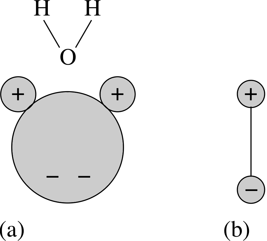
Figure 7 The water molecule (H²O). (a) The positions of the atoms. (The small atoms are the hydrogen atoms, as indicated by the orientation of the water molecule shown.) (b) The equivalent dipole.

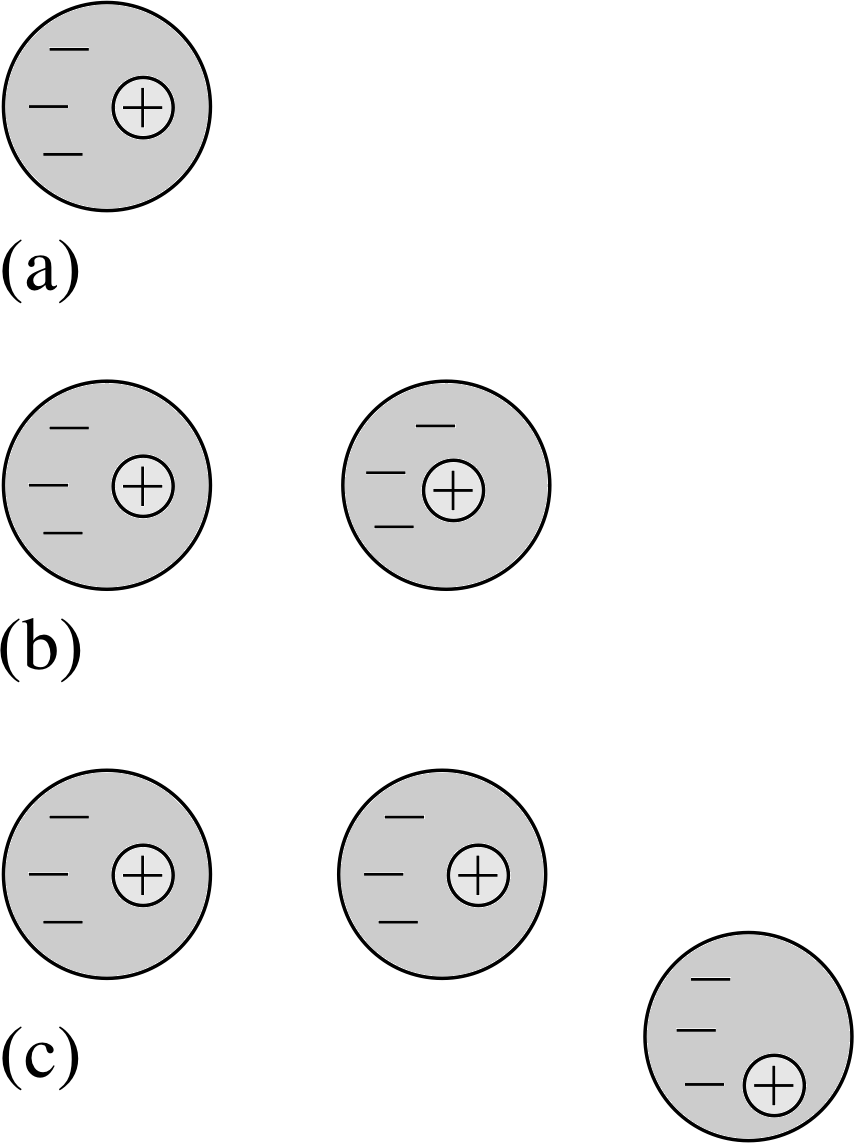
Figure 8 (a) An instantaneous asymmetry in the charge distribution of an atom gives rise to (b) an induced dipole in a nearby atom which reinforces the original dipole and also (c) induces a dipolar distribution in a third atom.

4 Electric potential and electric field

Calculations with vector quantities such as forces and fields can become very complicated, especially if vector addition has to be used repeatedly. This difficulty can be avoided sometimes by thinking in terms of energy (which is a scalar quantity) rather than force (which is a vector). This section introduces the related concepts of electrostatic potential energy and electric potential that are used in such situations.

4.1 Electrostatic potential energy

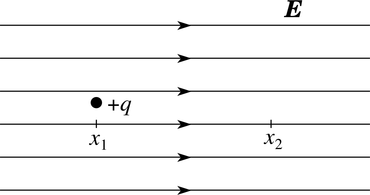
Figure 9 A positive charge +q in a uniform electric field E.

Figure 9 shows a particle of positive charge +q in a uniform electric field, i.e. in a field that has the same magnitude and direction at every point. Coordinates have been chosen in such a way that the field points along the x–axis, so its only non–zero component is E_x, and even that is the same everywhere due to the uniformity of the field. The charged particle is initially stationary, but it will be subject to an electrostatic force F_x = qE_x in the x–direction, so if free to move it will accelerate in the direction of the force in accordance with Newton’s second law of motion. i As a result of such motion the particle will gain kinetic energy. The kinetic energy E_kin gained in any movement, is equal to the work W done by the electrostatic force on the charge. i

In moving through a displacement ∆x, the work done will be qE_x∆x, so this will change the kinetic energy by an amount ∆E_kin given by:

∆E_kin = qE_x∆x(8) i

An alternative way of describing the same situation is to say that the charge possesses a certain amount of electrostatic potential energy (or electrical energy for short) which depends on its position in the field. The increase in kinetic energy is exactly balanced by a decrease in electrostatic potential energy so that the total energy change is zero and we may write

∆E_el + ∆E_kin = 0(9) i

So,∆E_el = −∆E_kin, but we already know that ∆E_kin = qE_x∆x

Hence, in a uniform field the change in electrostatic potential energy as a result of a displacement parallel to the field is:

∆E_el = −qE_x∆x(10)

Question T9

In an electron gun in a television set, the electrons which strike the screen to create the picture are accelerated by travelling a distance of 1.00 cm in a uniform electric field of 3.00 × 10⁴ N C⁻¹. Assuming the electrons are initially at rest, calculate (a) the potential energy lost by the electrons when they are accelerating and (b) their final speed. i

Answer T9

(a) Assuming the (negatively charged) electron is moving in the positive x–direction, the electric field must be directed in the negative x–direction.

Using ∆E_el = −qE_x∆x

∆E_el = −(−1.60 × 10⁻¹⁹ C) × (−3.00 × 10⁴ N C⁻¹) × 1.00 × 10⁻² m

i.e.∆E_el = −4.80 × 10⁻¹⁷ J (i.e. 300 eV)

The negative sign indicates that the potential energy has decreased during the journey.

(b) Using Equation 9,

∆E_el + ∆E_kin = 0(Eqn 9)

we can write

∆E_el + ½ mυ² = 0

So½ mυ² = −∆E_el

and$\upsilon = \sqrt{\dfrac{-2\Delta E_{\rm el}\os}{m}} = \rm \sqrt{\dfrac{-2\times(-4.8\times 10^{-17})}{9.1\times 10^{-31}}}\,m\,s^{-1}$

i.e.υ = 1.0 × 10² m s⁻¹ (to two significant figures)

For a charge moving in a non–uniform field E(r), the calculation of electrostatic potential energy is more complicated. As a first step towards finding the general expression for the potential energy of such a charge suppose that the motion is restricted to the x–direction, so we only have to worry about the field component in the x–direction, E_x(r). i We can imagine that the charge q moves in short steps of length ∆x that are small enough that E_x(r) can be regarded as constant for each step. The work done in a single small step starting at r will be ∆W = qE_x(r)∆x, and the total work done in moving from x₁ to x₂ will be approximately equal to the sum of the work in each small step, which we can write:

$\displaystyle W \approx \sum qE_x({\boldsymbol r})\,\Delta x$

This approximation will become increasingly accurate as the steps become smaller and smaller, with the consequence that in the limit as the steps become vanishingly small we can write

$\displaystyle W = \lim_{\Delta x \rightarrow 0}\left[\sum qE_x({\boldsymbol r})\Delta x\right] = q\lim_{\Delta x \rightarrow 0}\left[∑E_x({\boldsymbol r})\Delta x\right]$

Now, limits of sums of this kind are known as definite integrals, and are conventionally written as follows

$\displaystyle W = q \int_{x_1}^{x_2} E_x({\boldsymbol r})\,dx$(11)

hence$\displaystyle \Delta E_{\rm el} = -W = -q \int_{x_1}^{x_2} E_x({\boldsymbol r})\,dx$(12a)

In this case, we chose to consider motion in the x–direction so that we only had to consider a single component (E_x) of the non–uniform field. More generally, in two or three dimensions, the motion may be from any point r₁ to any other point r₂ and the movement may be along any pathway between those two points. For convenience we may consider this motion to be along x then along y and finally along z.

A simple extension of Equation 12a then leads to

$\displaystyle \Delta E_{\rm el} = -W = -q \left[ \int_{x_1}^{x_2} E_x({\boldsymbol r})\,dx +\int_{y_1}^{y_2} E_y({\boldsymbol r})\,dy + \int_{z_1}^{z_2} E_z({\boldsymbol r})\,dz\right]$

The quantity in square brackets can be expressed as the scalar product

$\displaystyle \int_{r_1}^{r_2} {\boldsymbol E}({\boldsymbol r}){\boldsymbol \cdot}\,d{\boldsymbol r}$

which is called a line integral. i

Under these circumstances the change in the electrostatic potential energy is given by:

$\displaystyle \Delta E_{\rm el} = -q\int_{{\boldsymbol r}_1}^{{\boldsymbol r}_2} {\boldsymbol E}({\boldsymbol r}){\boldsymbol \cdot}\,d{\boldsymbol r}$(12b) i

Like other integrals this is just a shorthand for a limit of a sum, though in this case the quantity being summed is the scalar product E(r) ⋅ ∆r where ∆r is a small displacement from one point to another on the relevant path from r₁ to r₂, and E(r) ⋅ ∆r = |E(r)||∆r|cosθ, where θ is the angle between E(r) and ∆r at any point r.

To show the importance of Equation 12b we will now use it to develop an expression for the electrostatic potential energy of a point test charge q in the field of another point charge Q. The non–uniform field of a fixed point charge, Q, at the origin of coordinates was introduced earlier, in a vacuum it takes the form

${\boldsymbol E}({\boldsymbol r}) = \dfrac{Qq}{4\pi\varepsilon r^2}\hat{\boldsymbol r}$Eqn (2)

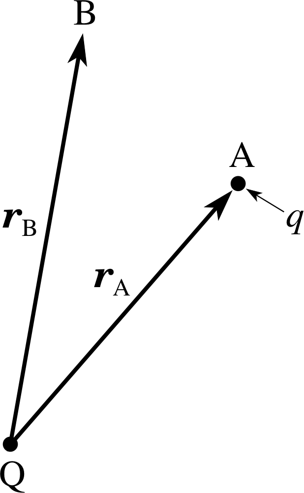
Figure 10 A charge q in a radial field due to a point charge Q.

This field is directed radially (towards or away from the origin) at all points. It follows that the work done by the electrostatic force when a particle moves from a point A to some other point B (Figure 10) is determined by the radial component of the field, E_r(r) = Q/(4πεr²), the charge q, and the difference in the radial coordinates r_A and r_B of A and B. (Note, it does not depend on the particular path that the charge follows from A to B.)

It follows from Equation 12b that in this case

$\displaystyle \Delta E_{\rm el} = -q\int_{r_{\rm A}}^{r_{\rm B}} E_r({\boldsymbol r}){\boldsymbol \cdot}\,dr$(12c) i

thus$\displaystyle \Delta E_{\rm el} = -q\int_{r_{\rm A}}^{r_{\rm B}} \dfrac{Q}{4\pi\varepsilon_0}\,dr = \dfrac{-qQ}{4\pi\varepsilon_0}\int_{r_{\rm A}}^{r_{\rm B}} \dfrac{1}{r^2}\,dr = \dfrac{-qQ}{4\pi\varepsilon_0}\left[\dfrac{-1}{r}\right]_{r_{\rm A}}^{r_{\rm B}}$

i.e.$\displaystyle \Delta E_{\rm el} = \dfrac{-qQ}{4\pi\varepsilon_0}\left(\dfrac{1}{r_{\rm B}}-\dfrac{1}{r_{\rm B}}\right)$(12d)

This expression for the change in the potential energy of the charge q between two positions is useful since it is such changes in potential energy that are physically meaningful. Nonetheless, it is sometimes convenient to be able to assign a definite value to the electrostatic potential energy of q when it is at some particular distance r from the origin. In order to do this we need to arbitrarily choose a reference point at which E_el = 0. The potential energy at any point is then the value of ∆E_el corresponding to the displacement from the reference point to the point of interest. When dealing with the field from a point charge, it is convenient to choose E_el = 0 where E(r) = 0, i.e. when r → ∞. We can then find the electrostatic potential energy of q at a distance r from Q by letting r_A → ∞ i and r_B = r in Equation 12d:

$\displaystyle E_{\rm el}\,(\text{of }q\text{ at }r) = \dfrac{-qQ}{4\pi\varepsilon_0}\dfrac1r$(13) i

Using Equation 12b,

$\displaystyle \Delta E_{\rm el} = -q\int_{r_1}^{r_2} {\boldsymbol E}({\boldsymbol r}){\boldsymbol \cdot}\,d{\boldsymbol r}$(Eqn 12b)

similar calculations may be carried out for any other electrostatic field, though the mathematics will usually be more complicated and the result will generally depend on the position vector r of q rather than just its magnitude r. For such general cases we can represent the electrostatic potential energy of the test charge by E_el(of q at r), but its value will still depend on some arbitrary choice of reference position

Question T10

A sphere carries a charge of +40 μC. A small particle with a charge of +2.0 μC is moved from a position outside the sphere and 1.0 m from its centre to a position 1.5 m from its centre.

(a) Without doing a calculation, decide whether the change in potential energy will be positive or negative.

(b) Calculate the change in potential energy. Will it make any difference if the particle moves in a straight line between the two positions or follows some complicated path?

Answer T10

(a) Both charges are positive, so the Coulomb force is repulsive. Therefore a positive quantity of work is done by the Coulomb force on the particle as it moves further from the sphere. From Equation 9, this means that the change in E_el will be negative.

(b) $\Delta E_{\rm el} = \dfrac{Qq}{4\pi\varepsilon_0}\left(\dfrac{1}{r_2}-\dfrac{1}{r_1}\right)$

so$\Delta E_{\rm el} = \rm \dfrac{40\times 10^{-6}\times 2.0\times 10^{-6}}{4\pi\times 8.85\times 10^{-12}}\left(\dfrac{1}{1.5}-\dfrac{1}{1.0}\right) = -0.24\,J$

The path taken by the particle makes no difference (because the force is conservative). The change in potential energy depends only on the initial and final positions and not on what happens in between.

Question T11

What is the electrical potential energy of the electron in a hydrogen atom as described in Question T1?

Answer T11

From Equation 13,

$\displaystyle E_{\rm el}\,(\text{of}~q~\text{at}~r) = \dfrac{-qQ}{4\pi\varepsilon_0}\dfrac{1}{r}$(Eqn 13)

$\Delta E_{\rm el} = \rm \dfrac{-\left(1.6\times 10^{-19}\right)^2}{4\pi\times 8.85\times 10^{-12}\times 5\times 10^{-11}}\,J = -4.6\times 10^{-18}\,J$

4.2 Electric potential: definition and representation

In much the same way that we defined the electric field at any point in terms of the force per unit positive charge, it is useful to define a quantity, called the electric potential, which represents the potential energy per unit charge that a test charge would have at any point:

$V({\boldsymbol r}) = \dfrac{E_{\rm el}\,(\text{of }q\text{ at }r)}{q}$(14) i

Note that like the electric field, the electric potential can be simultaneously assigned a value at every point, but V(r), unlike the electric field, is a scalar quantity.

In one dimension, the difference in potential between two positions x₁ and x₂ is (from Equation 12a):

$\displaystyle \Delta E_{\rm el} = -W = -q \int_{x_1}^{x_2} E_x({\boldsymbol r})\,dx$(Eqn 12a)

$\displaystyle \Delta V = -\int_{x_1}^{x_2} E_x\,dx$(15a)

and in three dimensions (from Equation 12b):

$\displaystyle \Delta E_{\rm el} = -q\int_{{\boldsymbol r}_1}^{{\boldsymbol r}_2} {\boldsymbol E}({\boldsymbol r}){\boldsymbol \cdot}\,d{\boldsymbol r}$(Eqn 12b)

$\displaystyle \Delta V = -\int_{{\boldsymbol r}_1}^{{\boldsymbol r}_2} {\boldsymbol E}({\boldsymbol r}){\boldsymbol \cdot}\,d{\boldsymbol r}$(Eqn 15b)

As with potential energy, we can arbitrarily define some point to have zero potential and then use Equation 15b to work out the potential at any other point. In the particular case of a point charge Q fixed at the origin, it is usual to choose V = 0 when r → ∞, then for any point at a distance r from Q

$V(r) = \dfrac{Q}{4\pi\varepsilon_0 r}$(16)

Since a spherically symmetric charge distribution produces the same external electrical effects as a point charge at its centre, Equation 16 also describes the potential at or beyond the surface of a conducting sphere that carries a net charge Q.

Electric potential is such a frequently used concept that its SI unit has been given a special name – the volt (V). Thus 1 V = 1 J C⁻¹. We are all familiar with this unit from its association with mains electricity, batteries, etc. Indeed differences in electric potential are often called voltages.

✦ Use Equation 14,

$V({\boldsymbol r}) = \dfrac{E_{\rm el}\,(\text{of }q\text{ at }r)}{q}$(Eqn 14)

to write down an expression for the change in electric potential energy ∆E_el when a particle with charge q moves through a potential difference ∆V.

✧ ∆E_el = q∆V

We are sometimes interested in the behaviour of individual electrons or ions in electric fields (as in the electron gun of Question T9). A single electron moving through a potential difference of, say, 2000 V has ∆E_el = 2000 J C⁻¹ × 1.602 × 10⁻¹⁹ C = 3.204 × 10⁻¹⁶ J – a very small energy change. Rather than always working in joules and having to deal with such very small numbers, it is convenient to introduce a different energy unit.

One electronvolt (eV) is defined as the change in the electrostatic potential energy of a single electron when it moves through a potential difference of 1 V. 1 eV = 1.602 × 10⁻¹⁹ C × 1 V = 1.602 × 10⁻¹⁹ J.

The electronvolt is not an SI unit, but it is very widely used to measure small energies. i To find ∆E_el in eV for a single charged particle moving through a potential difference, you simply multiply its charge (measured in units of e, not in Coulombs) by the potential difference (measured in volts). For example, an electron moving through a potential difference of 2000 V will change its electrical potential energy by 2000 eV (often written 2 keV). Similarly, if an oxygen ion of charge 2e, formed from an oxygen atom that has lost two of its electrons, moves through 2000 V then ∆E_el is 4 keV.

Question T12

For a battery, the ‘negative’ terminal is usually taken to be at zero potential. If a 12 V car battery is connected to two plates within a vacuum, and an electron released from the negative plate travels to the positive plate, what will be the change in the electron’s electrostatic potential energy (give your answer in eV and in J)?

Answer T12

∆E_el = −12 eV = 12 × −1.602 × 10⁻¹⁹ J = −1.92 × 10⁻¹⁸ J

The importance of the potential

One of the great advantages of dealing with potentials is the ease with which they may be added together. The electric potential at a point in space due to a number of charges is simply the sum of the potentials due to the individual charges. Thus for a distribution of point charges, Equation 16,

$V(r) = \dfrac{Q}{4\pi\varepsilon_0 r}$(Eqn 16)

can be used repeatedly to calculate the total potential at any point.

The scalar nature of the potential means that it is often relatively straightforward to determine the potential due to a given charge distribution.

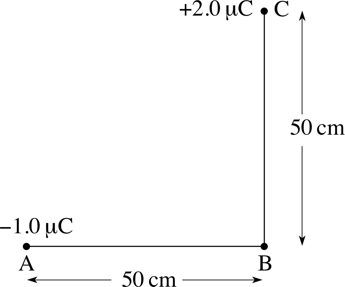
Figure 11 See Question T13.

Question T13

Calculate the electric potential at point B in Figure 11 due to the charges at A and C.

Answer T13

$V = \dfrac{q_{\rm A}}{4\pi\varepsilon_0 r_{\rm AB}} + \dfrac{q_{\rm C}}{4\pi\varepsilon_0 r_{\rm CB}} = \dfrac{1}{4\pi\varepsilon_0}\left(\dfrac{q_{\rm A}}{r_{\rm AB}}+\dfrac{q_{\rm C}}{r_{\rm CB}}\right)$

so$V = \rm 8.99\times10^9\left(\dfrac{-1.0\times 10^{-6}}{0.50}+\dfrac{-2.0\times 10^{-6}}{0.50}\right)\,V$

i.e.V = 1.8 × 10⁴ V

The other crucial feature of the potential V(r) is that it can be used to derive the associated electrostatic field. We will introduce the relationship between the field and the potential by considering a deliberately simple case in which the electric potential V(r) depends on x but is actually independent of y and z. Under these circumstances we may represent the potential by V(x). If a charge q undergoes a small displacement from x to x + ∆x, the electrostatic force that acts throughout the displacement will be approximately given by qE_x(x), and the corresponding change in electrostatic potential energy of the charge will be ∆E_el ≈ −qE_x(x)∆x. It follows that the potential difference between x and x + ∆x is ∆V = ∆E_el/q ≈ −E_x(x)∆x. Rearranging this we see that

$E_x(x) ≈ -\dfrac{\Delta V}{\Delta x}$

This approximation will become increasingly accurate as ∆x is reduced, with the result that in the limit as ∆x becomes vanishingly small

$\displaystyle E_x(x) = -\lim_{\Delta x\rightarrow 0}\left(\dfrac{\Delta V}{\Delta x}\right)$

Now the limit on the right–hand side defines the gradient of the graph of V against x, that is the derivative of V(x) with respect to x:

$E_x(x) = -\dfrac{dV}{dx}$(17) i

So, the x–component of the electric field is given by minus the gradient of the potential.

Equation 17 emerged from the study of a deliberately simplified case; more generally the potential will depend on x, y and z, and we will have to work out all three components of the electric field at each point r. However, similar principles apply even though the mathematics is more complicated.

We can summarize this:

1: Once the electric potential is known in some region it is always possible to determine the corresponding electrostatic field by taking appropriate derivatives of the potential. The component of the electric field in any direction is minus the potential gradient in that direction.
2: The direction of the electric field at a point is given by the direction in which the potential decreases most rapidly.
3: The magnitude of the electric field at a point is the magnitude of the maximum potential gradient, measured along the direction of the electric field.

Equation 17 also shows that the SI unit of electric field can be written in the form V m⁻¹ which emphasizes the fact that the field is related to the potential gradient.

✦ Show that 1 V m⁻¹ = 1 N C⁻¹.

✧ By definition, 1 V = 1 J C⁻¹ and 1 J = 1 N m. Therefore 1 V m⁻¹ = 1 J C⁻¹ m⁻¹ = 1 N m C⁻¹ m⁻¹ = 1 N C⁻¹.

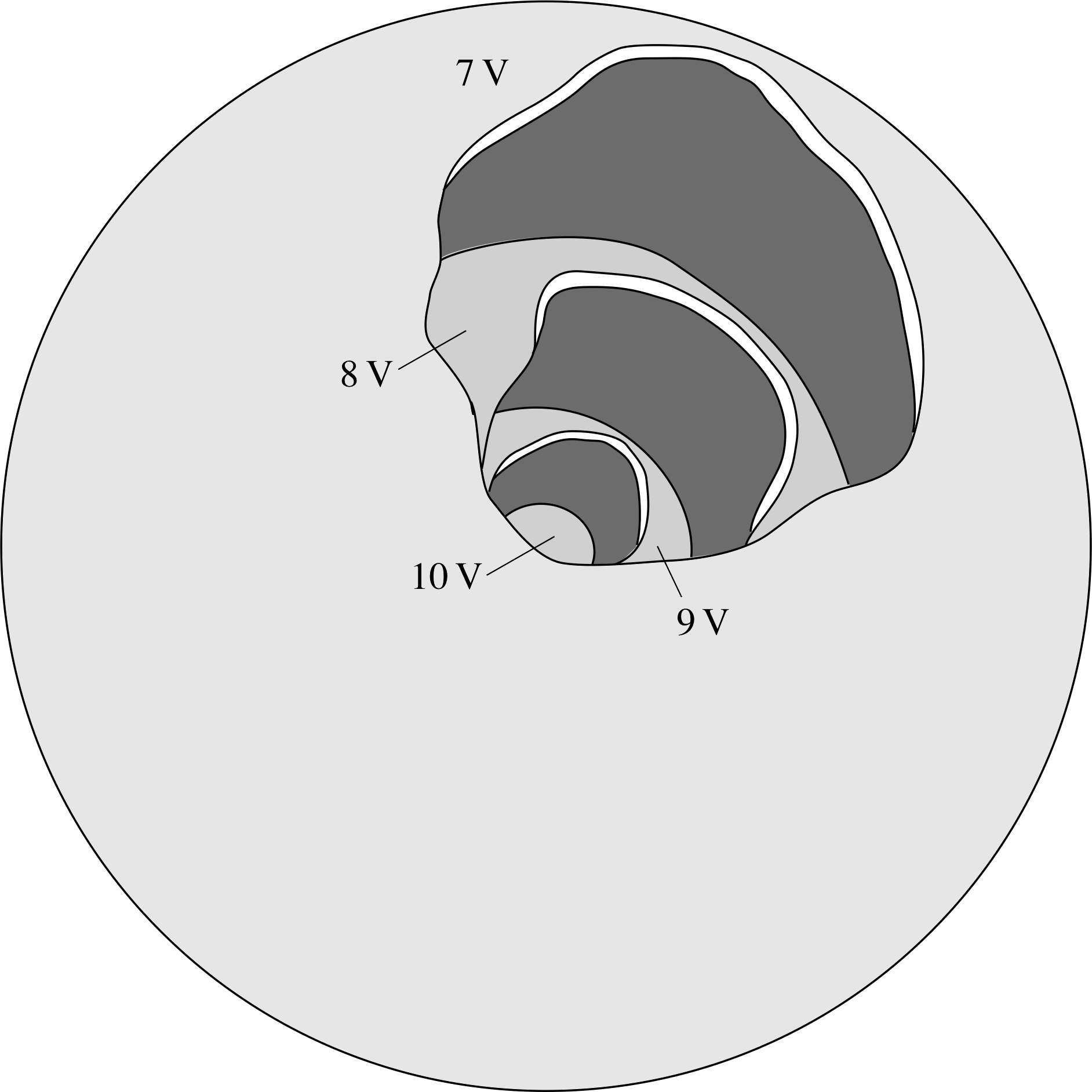
Figure 12 Equipotential surfaces surrounding a point charge.

Equipotentials and the representation of potentials

In Subsection 3.1, you saw how electric field lines provide a useful means of visualizing electric fields. A different kind of visualization can be achieved using the concept of electric potential. In two dimensions a line passing only through points of 8 V equal electric potential is known as an equipotential line, and in three dimensions we can similarly define equipotential surfaces. From point 2 above we can see that the electric field at any point must always be perpendicular to such lines or surfaces.

Figure 12 shows equipotential surfaces surrounding a point charge. The surfaces are separated by equal intervals of potential. The surfaces form concentric spheres showing that the field must be radial everywhere.

The fact that the surfaces crowd together near the charge shows that the field is stronger in this region. The fact that the field is related to minus the gradient of the potential shows that the field points away from regions of relatively high potential, towards regions of lower potential.

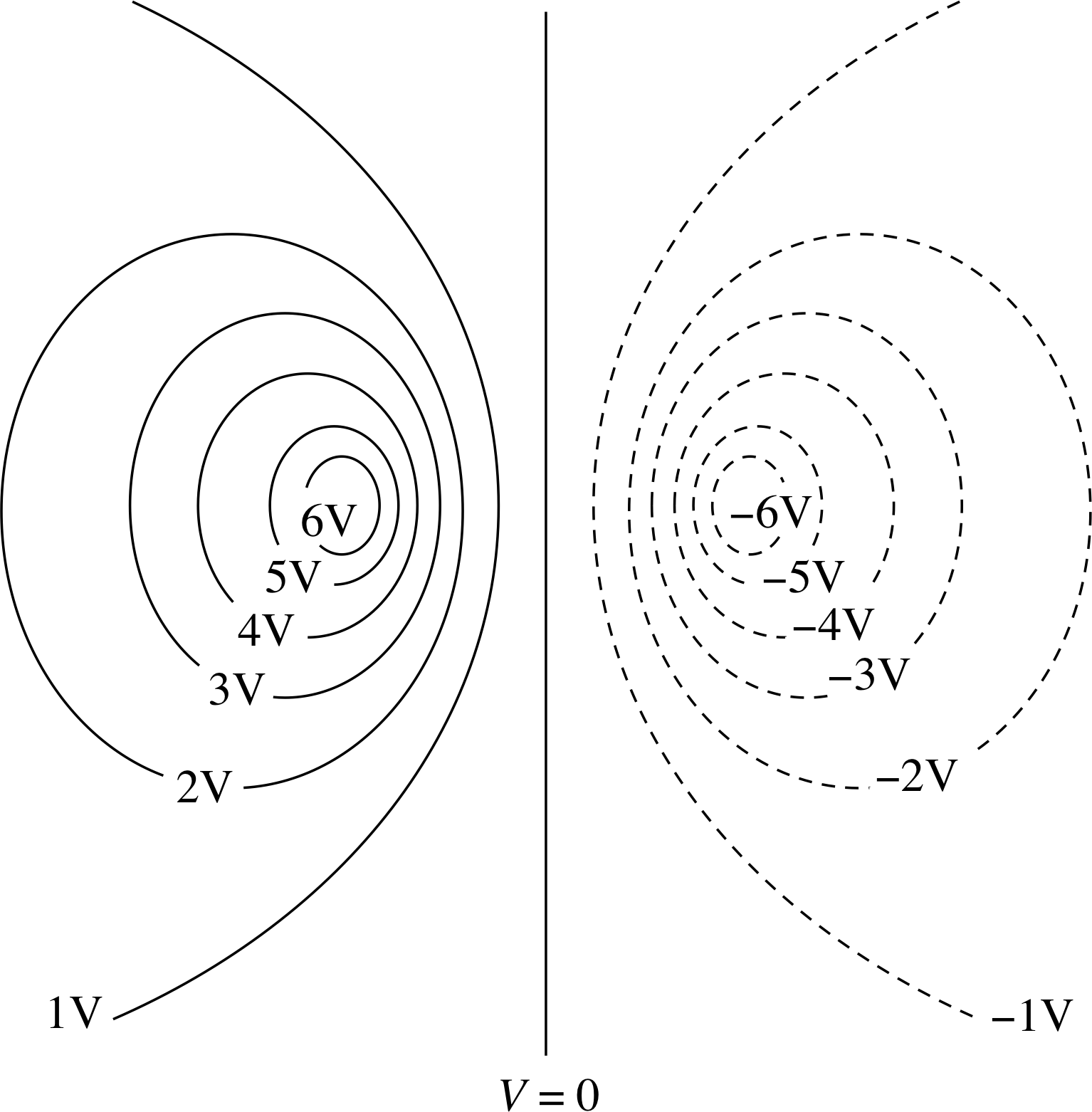
Figure 13 See Question T14.

Question T14

Figure 13 shows an equipotential plot for a particular charge distribution. In Figure 13:

(a) indicate positions of positive and negative charge;

(b) say whether charges are approximately the same size or, if not, which is the bigger;

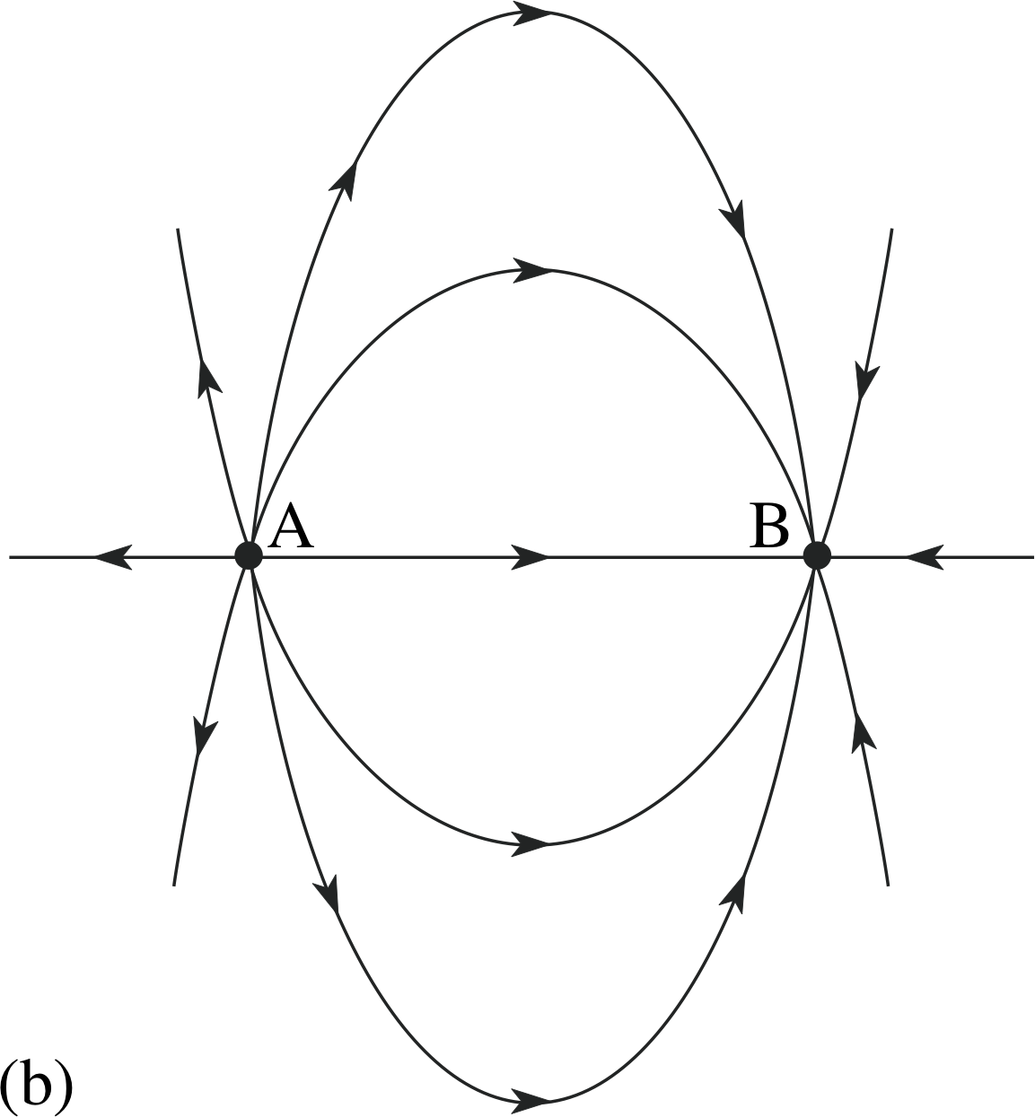
Figure 4b See Answer T14.

Answer T14

(a) There must be a positive charge within the maximum positive potential contour and a negative charge within the maximum negative potential contour.

(b) The size of the positive and negative maxima are the same so the charges must have the same magnitude.

(c) The electric field lines are everywhere perpendicular to the equipotentials. The field lines will therefore look like Figure 4b, the field of an electric dipole.

4.3 Millikan’s experiments to measure e

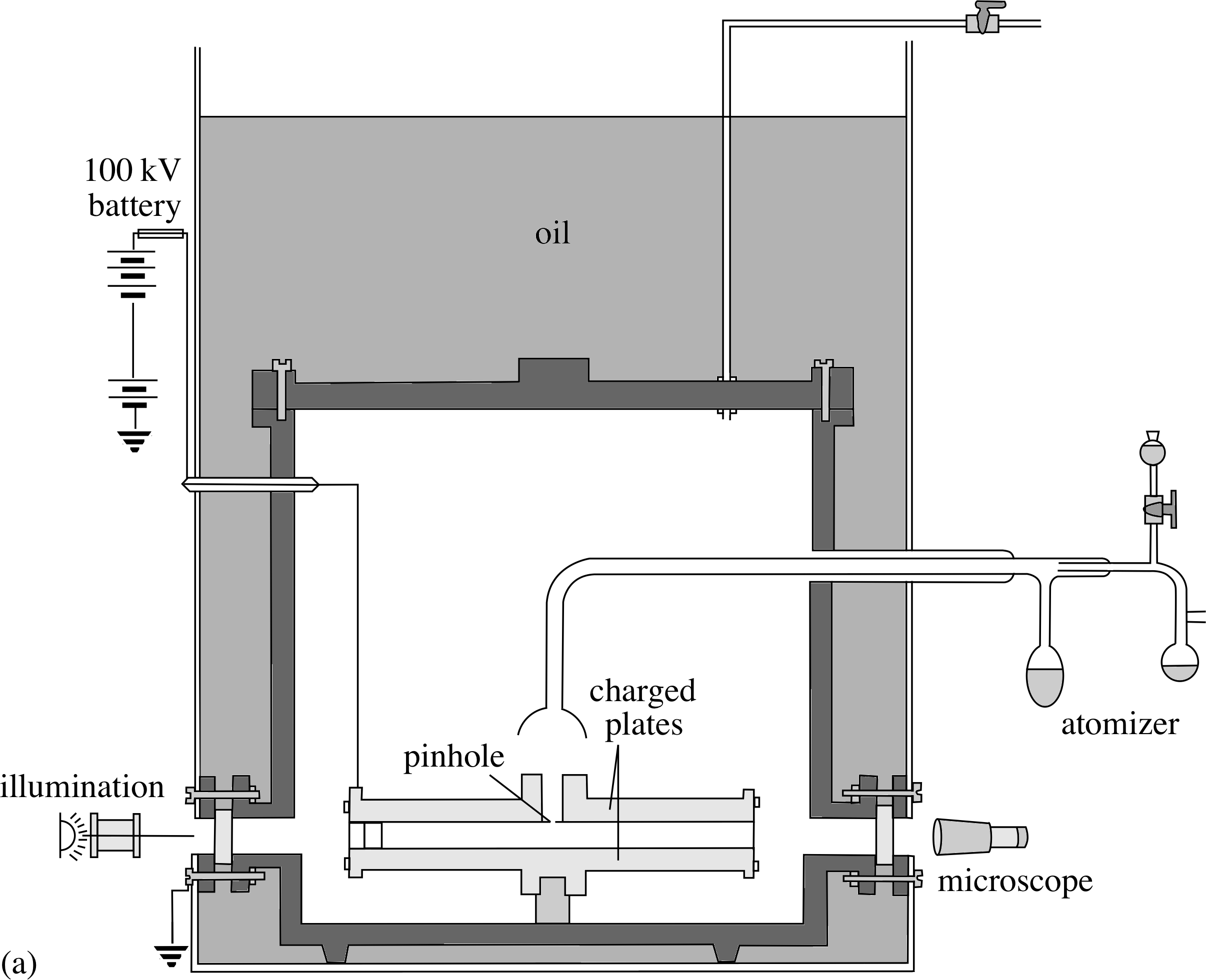
Figure 14a Schematic diagram of Millikan’s apparatus.

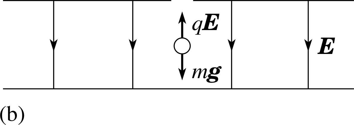
Figure 14b The behaviour of a negatively charged oil droplet between the charged plates.

In Subsection 2.1 we referred to Millikan’s experiments which supplied evidence for the quantization of charge and which provided a value for e, the electronic charge. To arrive at his results, Millikan studied the behaviour of small charged oil droplets in an electric field. Figure 14a shows a schematic diagram of his apparatus.

A fine spray of oil droplets is produced at the top of the apparatus and, in the process, the droplets become charged by friction. Falling under gravity, i some of the charged droplets enter the illuminated space between two metal plates that have an adjustable potential difference between them.

The experimenter, observing through the microscope, selects one of the droplets and adjusts the potential difference so that the droplet remains stationary in mid air; the downward force due to gravity on the droplet then being exactly balanced by an upward electrostatic force (Figure 14b). The electric field between the plates is uniform, so (from Equation 17)

$E_x(x) = -\dfrac{dV}{dx}$(Eqn 17)

it has magnitude

E = V/d(18)

where V is the balancing potential difference and d the distance between the plates.

The magnitude of the electrostatic force on a droplet of charge magnitude |q| is F_el = |q|E (from Equation 2),

${\boldsymbol E}({\boldsymbol r}) = \dfrac{Qq}{4\pi\varepsilon r^2}\hat{\boldsymbol r}$(Eqn 2)

so for a stationary droplet

|q|V/d = mg(19)

The mass m of the droplet can be found either by measuring its diameter (by observing it against a graduated scale) and calculating m using the density of the oil, or by measuring the droplet’s terminal velocity i as it falls through the air in the absence of any electric field. Knowing V, d, g and m for any particular droplet, Equation 19 can be used to determine the magnitude and sign of q.

Millikan carried out his experiments over several years, and introduced various refinements to improve accuracy. He used a non–volatile oil, so that the mass of a droplet would not change due to evaporation, and convection currents were reduced by enclosing the apparatus in a constant temperature oil bath. In a further improvement, he used X–rays to alter the charge so that he could make several different charge measurements on any one droplet. i

By repeating his experiments with a very large number of droplets, Millikan found that the charge magnitude on a droplet was always a whole number multiple of a basic charge e, where e = 1.6 × 10⁻¹⁹ C (to two significant figures).

Question T15

(a) What could you deduce about the basic unit of charge if you measured the magnitude of the charges on some oil drops to be 3.2 × 10⁻¹⁹ C, 6.4 × 10⁻¹⁹ C and 1.28 × 10⁻¹⁸ C?

(b) How might your conclusion be affected if you measured a charge magnitude of 4.8 × 10⁻¹⁹ C?

Answer T15

(a) The basic unit would be 3.2 × 10⁻¹⁹ C, since the measured charges are 1×, 2× and 4× this amount – the basic unit could be smaller, but these results do not require it to be.

(b) This charge is not a whole number times 3.2 × 10⁻¹⁹ C, but if the basic unit is 1.6 × 10⁻¹⁹ C, then all the results are whole number multiples, i.e. 2×, 4×, 8× and 3×. The point about Millikan’s experiments is that he never needed to use a basic charge that was any smaller than 1.6 × 10⁻¹² C to interpret his results.

Question T16

An oil drop of mass 9.8 × 10⁻¹⁵ kg is suspended between two plates 1.0 cm apart with a potential difference of 2000 V across the gap. If the drop is negatively charged due to an excess of electrons, how many such electrons must there be on the drop? i

Answer T16

From Equation 19,

|q|V/d = mg(Eqn 19)

|q| = mgd/V = 9.8 × 10⁻¹⁵ kg × 9.81 N kg⁻¹ × 1.0 × 10⁻² m/2000 V = 4.8 × 10⁻¹⁹ C

i.e.q = −3 × 1.6 × 10⁻¹⁹ C, so the drop must have three excess electrons.

5 Point discharge and thunderstorms

5.1 Point discharge

Lightning tends to strike tall pointed objects (such as trees and church spires). We can understand why by thinking about the electric field around an irregularly–shaped charged conductor.

If a conductor is charged, the excess charge will distribute itself on the surface so as to minimize the repulsive forces between like charges – it moves until there is no electric field within the conductor. We can put this another way: charge will move so as to minimize its electric potential energy – it will move until there is no potential difference between the various parts of the conductor. i It follows that:

The surface of a conductor will be an equipotential surface.

This has some important consequences for the associated field and charge distribution.

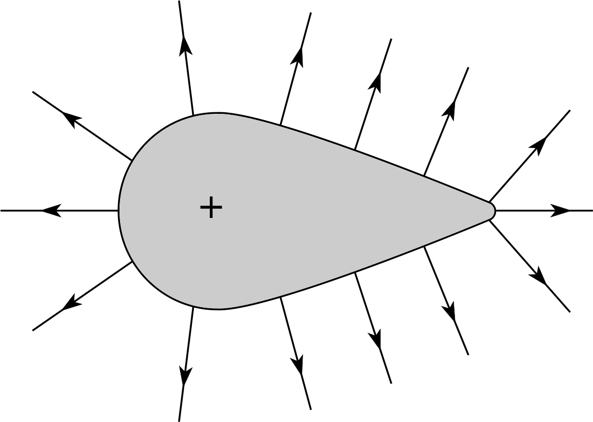
Figure 15 Field lines around an irregularly–shaped conductor that carries a net positive charge.

✦ Figure 15 shows the field lines meeting a positively–charged conductor. i Whereabouts is the field outside the conductor strongest? And whereabouts on the conducting surface is the greatest concentration of charge?

✧ The field is strongest where the field lines are converging most sharply, i.e. around the pointed end. The greatest charge concentration must be where the field is strongest, i.e. also at the point.

Although most of the atmosphere consists of neutral atoms, there are always a few stray electrons and ions, and these charged particles are available to be accelerated by an electric field. Around a charged object such as that in Figure 15, the movement of charge will be greatest in the air near the pointed end where the field is strongest. Positive ions are repelled from the point, and electrons are attracted to it, so the conductor becomes neutralized by charge of the opposite type – the process is known as point discharge.

A conductor with any sharp corners will lose its charge more rapidly than one whose surface is a smooth curve. This is one of the reasons why scientific equipment used in the study of electrostatics often includes spherical conductors (Figure 16).

5.2 Lightning and thunder

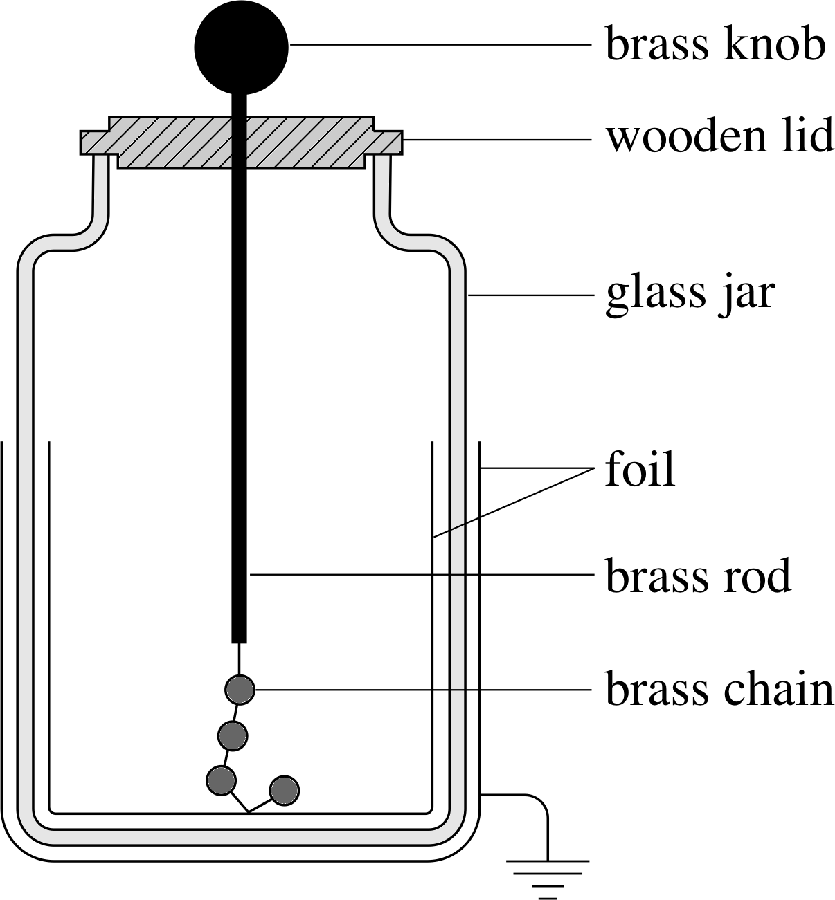
Figure 16 A schematic diagram of a Leyden jar (an antique electrical storage device) with a spherical conductor to minimize point discharge.

We now have the tools with which to tackle the questions about lightning that were posed in the introduction to this module. First of all, what is lightning?

As mentioned in Subsection 5.1, there are always a few charged particles in the air that are available to be accelerated by an electric field. If the field is strong enough they can be accelerated to such high energies that when they collide with atoms they liberate more electrons. The ions and freed electrons are then accelerated in their turn, colliding with more atoms and creating a cascade of charged particles. This converts very large amounts of electrical potential energy into kinetic energy in a very short time giving rise to intense local heating of the air.

Temperatures can reach 3 × 10⁴ K which is about five times hotter than the surface of the Sun! We see this as a visible flash. The sudden heating has another effect: it causes the air to expand explosively generating a shock wave which creates the sound of thunder.

The electric field required to cause electrical breakdown of the air in this manner is of the order of 3 × 10⁶ V m⁻¹. i

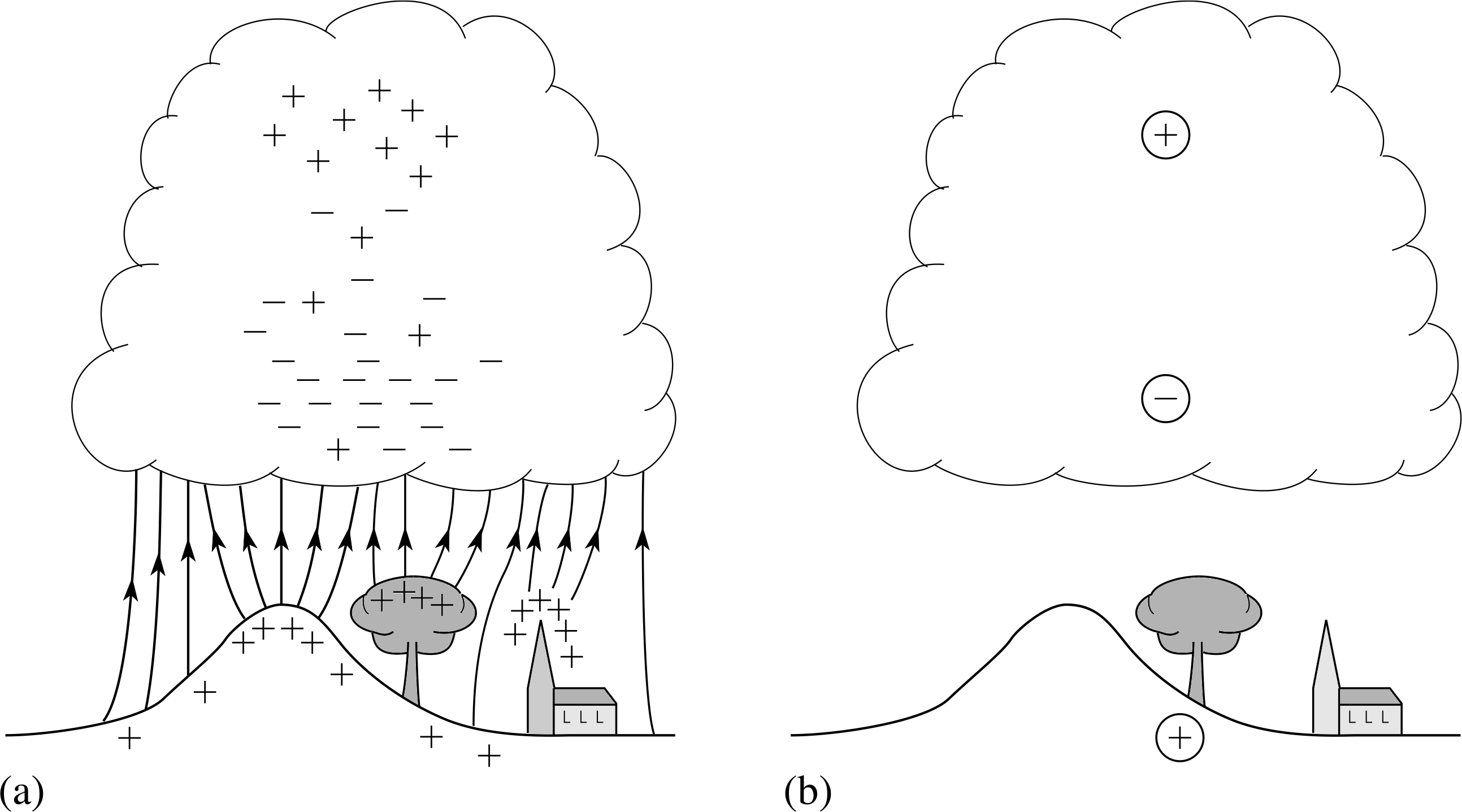
Figure 17 Charge separation in a thunder cloud. (a) The distribution of charges. Field lines between the cloud and Earth are also shown. (b) The charge distribution replaced by point charges.

We know that large fields must be associated with large concentrations of charge. It is apparent therefore that thunderclouds must be highly charged. How does this happen?

The precise mechanism of the charging process is not fully understood but it has to do with the strong rising currents of moist air associated with thunderstorm activity. Ice crystals formed within the cloud fall through a spray of warm, rising water droplets and become negatively charged leaving the droplets with a net positive charge.

This results in a charge separation in the cloud as shown in Figure 17a.

Although the distribution of charges is complex, we can get a rough idea of what is going on by assuming the positive and negatively charged regions are spherical and replacing them with point charges. A typical thunderstorm modelled in this way is shown in Figure 17b. It has negative and positive charges of roughly 50 C at heights of 5 km and 10 km, respectively.

Question T17

Using the information above calculate the field strength (a) halfway between the dipole charges in the cloud shown in Figure 17b and, (b) at the position of the Earth’s surface due to the dipole, assuming the presence of the Earth does not affect the calculation. (It has negative and positive charges of roughly 50 C at heights of 5 km and 10 km, respectively.}

Answer T17

(a) The field halfway between the charges will be just twice the field due to one of the charges. The magnitude will be given by

$E_{\rm cloud} = \dfrac{2Q}{4\pi\varepsilon_0 r^2} = \rm \dfrac{2\times 50}{4\pi\times 8.85\times 10^{-12}\times\left(2500\right)^2}\,V\,m^{-1}$

The direction of this field will be vertically downwards.

(b) At the Earth’s surface

$E_{\rm surface} = \left[\dfrac{50}{4\pi\varepsilon_0\left(5\times 10^3\right)^2}-\dfrac{50}{4\pi\varepsilon_0 \left(10\times 10^3\right)^2}\right]\,{\rm V\,m^{-1}} = \rm 1.3\times 10^4\,V\,m^{-1}$

The direction of this field will be vertically upwards.

The assumption in the last part of Question T17 is not in fact correct. The Earth behaves as a good conductor and the negative charges at the base of the cloud induce a net positive charge in the Earth’s surface. The effect of this is to double the calculated value of E at the Earth’s surface. There will also, of course, be local variations. As a conductor, the Earth’s surface is an equipotential. For high ground, the potential difference between the Earth and the cloud base will be the same as for low ground, but the distance between them will be shorter giving a larger potential gradient (see Figure 17a).

Added to this, as mentioned in Subsection 5.1, the ground charge will tend to concentrate at regions of high curvature. Thus fields become intensified near pointed objects. Even so, fields close to the Earth are usually less than the required figure of ~3 × 10⁶ V m⁻¹ for the initiation of lightning. Most lightning flashes begin with localized high fields inside the cloud. Once the initial ionization starts, the ‘flash’ moves in short bursts, at each stage following the local potential gradient. This occurs both for flashes between the charges in the cloud and between the base of the cloud and Earth. Typically 30 C of charge is transferred in less than 1 second.

The other question posed in the Introduction is whether the advice given to mountaineers in the Mountain Leadership Guide makes sense. The electric field close to the Earth is stronger near high ground and pointed or sharply curving objects. Consequently, the advice to avoid trees, boulders and peaks and to crouch down or squat is good. Figure 17a shows that the concentration of field lines on peaks and projections means the field some distance away will be reduced – as a rule of thumb, find a position about the same distance away as the projection is high.

When lightning strikes the ground there is an enormous transfer of charge in a very short time. This means there are very large fields through the ground in the vicinity of the strike. If you have two points of contact with the ground separated by a distance ∆x, the potential difference between those points is given by ∆V = E∆x. So the greater the separation between the points of contact, the greater potential difference. As your body is a good conductor, charge will flow through you between the points of contact with the ground. You minimize the danger by keeping your points of contact as close together as possible and making sure that the conducting path does not include your heart or brain. You can achieve this by squatting and keeping your hands off the ground.

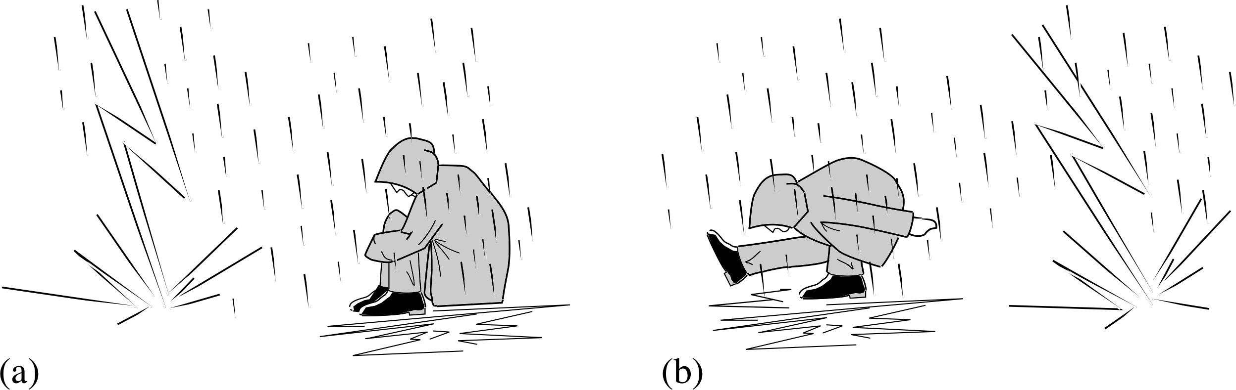
Figure 18 How to minimize the danger from a lightning strike. (a) The recommended position and (b) the optimum position.

Figure 18a shows a sensible position. You could improve on the Mountain Leadership Guide advice by maintaining only one point of contact with the ground, while still remembering to keep as low as possible

This is illustrated in Figure 18b – but maybe being struck by lightning would be preferable to keeping this up for any length of time!

6 Closing items

6.1 Module summary

1

There are two kinds of electric charge labelled positive and negative. Charge is quantized in units of e where e = 1.603 × 10⁻¹⁹ C. The total charge in the universe is a conserved quantity.

2

Materials can be broadly classified as electrical conductors or insulators, according to the ease with which charge moves within them. (There is also a class of materials known as semiconductors which behave as conductors in some circumstances and insulators in others.)

3

Transfer of charge between two initially neutral objects made of appropriate materials may be effected by rubbing the two objects together. Conductors may be charged by electrostatic induction.

4

The electrostatic force between charged particles (or spherically symmetric bodies) is governed by Coulomb’s law:

${\boldsymbol F}_{21} = \dfrac{q_1 q_2}{4\pi\varepsilon r^2}\hat{\boldsymbol r}$(Eqn 1c)

where r^{^}/|r| and ε = ε₀ε_r.

The electrostatic force due to a distribution of charges is the vector sum of the electrostatic forces of the individual charges.

5

The electric field E at any point is the electrostatic force per unit (positive) charge that would be experienced by a test charge placed at that point:

${\boldsymbol E}(x,\,y,\,z) = \dfrac{F_{\rm el}~(\text{on}~q~\text{at}~(x,\,y,\,z))}{q}$

The electric field at any point specified by r = (x, y, z) due to a point charge Q at the origin is

${\boldsymbol E}({\boldsymbol r}) = \dfrac{Qq}{4\pi\varepsilon r^2}\hat{\boldsymbol r}$(Eqn 2)

6

Field lines are a useful, semiquantitative way of representing the electric field in a region of space. They emerge from positive charges, point in the direction of the electric field at any point, and are drawn in such a way that their density in any region is proportional to the strength of the electric field in that region.

7

An electric dipole is a pair of charges with equal magnitude and opposite sign separated by a small displacement. The dipole moment is the product of the charge magnitude and separation. Coulomb forces between molecular or atomic dipoles (called van der Waals forces) are responsible for intermolecular bonding in many solids.

8

The change in electrostatic potential energy of a charge q in an electric field E(r) when it is moved from r₁ to r₂ is the negative of the work done by the electrostatic force during the displacement. It is independent of the path followed from r₁ to r₂ and is given by

$\displaystyle \Delta E_{\rm el} = -q\int_{{\boldsymbol r}_1}^{{\boldsymbol r}_2} {\boldsymbol E}({\boldsymbol r}){\boldsymbol \cdot}\,d{\boldsymbol r}$(Eqn 12b)

For a point charge q at a distance r from a charge Q we can say that

$\displaystyle E_{\rm el}\,(\text{of}~q~\text{at}~r) = \dfrac{-qQ}{4\pi\varepsilon_0}\dfrac{1}{r}$(Eqn 13)

provided we adopt the arbitrary convention that E_el = 0 where r → ∞.

9

For any charge distribution, the electric potential at any point in space is the electrostatic potential energy per unit charge that a test charge would have at that point

$\displaystyle V({\boldsymbol r}) = \dfrac{E_{\rm el}\,(\text{of}~q~\text{at}~r)}{q}$(Eqn 14)

For a point charge q at a distance r from a charge Q, V(r) depends only on r = |r| and may be written

$V(r) = \dfrac{Q}{4\pi\varepsilon_0 r}$(Eqn 16)

provided E_el = 0 where r → ∞.

10

The unit of electric potential is the volt (V), where 1 V = 1 J C⁻¹. The electronvolt (eV) is the change in the electrostatic potential energy of a single electron when it moves through a potential difference of 1 V. Since ∆E_el = q∆V, 1 eV = 1.602 × 10⁻¹⁹ C × 1 V = 1.602 × 10⁻¹⁹ J.

11

The (scalar) electric potential due to a distribution of charge is often relatively easy to determine. At any point, the component in any direction of the corresponding electric field is minus the gradient of the potential, in that direction. In the case of an electric field that varies only in the x–direction, V depends only on x and

$E_x(x) = -\dfrac{dV}{dx}$(Eqn 17)

12

Equipotential lines are lines passing only through points of equal potential; equipotential surfaces are surfaces passing only through points of equal potential. The electric field is everywhere perpendicular to equipotential lines and surfaces and points in the direction in which the potential decreases most rapidly.

13

The surface of a conductor will be an equipotential surface.

6.2 Achievements

Having completed this module, you should be able to:

A1: Define the terms that are emboldened and flagged in the margins of the module.
A2: Explain how objects may be charged by contact and by induction.
A3: State and use Coulomb’s law.
A4: Explain the origin of van der Waals forces in terms of forces between induced dipoles.
A5: Explain the concept of electric field, write down an expression for the field due to a point charge and describe the electric fields that arise in a range of simple situations (e.g. the uniform electric field).
A6: Describe the field due to an electric dipole and say how it differs from that due to a point charge.
A7: Perform simple calculations involving electric fields.
A8: Draw and interpret electric field line patterns for simple charge distributions.
A9: Distinguish between electrostatic potential energy and electric potential and perform simple calculations based on these concepts.
A10: Describe the relationship between electric field and electric potential, and use it in cases where the potential depends on only one variable.
A11: Explain the significance of equipotentials and their relationship to field lines.
A12: Explain the phenomenon of point discharge in terms of charge, field and potential.
A13: Explain in terms of charge, field and potential the cause of lightning and simple precautions which can be taken to minimize risk of injury due to lightning strikes.

Study comment You may now wish to take the following Exit test for this module which tests these Achievements. If you prefer to study the module further before taking this test then return to the topModule contents to review some of the topics.

6.3 Exit test

Study comment Having completed this module, you should be able to answer the following questions each of which tests one or more of the Achievements.

Question E1 (A2 and A3)

A spherical conductor carrying a charge of 4.00 × 10⁻⁵ C is momentarily connected to a second, identical, initially neutral, spherical conductor. After this, the spheres are positioned a certain distance apart where the force between them is measured as 0.200 N. Calculate their separation. Is the force between the spheres repulsive or attractive?

Answer E1

During contact we can assume that the charge is evenly distributed between the two conductors. So when they are separated each has a charge of 2 × 10⁻⁵ C. In this case, the magnitude of the force between them is

$F = \dfrac{Q^2}{4\pi\varepsilon_0 r^2}$

thus$r = \dfrac{Q}{\sqrt{4\pi\varepsilon_0 F\os}} = \rm \dfrac{2.00\times 10^{-5}}{\sqrt{4\pi\times 8.85\times 10^{-12}\times0.200}}\,m$

i.e.r = 4.24 m

Since the charge on both spheres has the same sign, the force will be repulsive. (Reread Subsections 2.2 and 2.3 if you had difficulty with this question.)

Figure 19 See Question E2.

Question E2 (A5, A7, A9 and A10)

Two point charges A and B of +2Q and +Q, respectively, are separated by a distance D (Figure 19).

(a) Show that there is a point on the line joining the two charges, at a distance of $\left(\dfrac{\sqrt{2\os}}{1+\sqrt{2\os}}\right)D$ from A, where the field is exactly zero.

(b) Show that the electric potential at this point is $\dfrac{Q(3 + 2\sqrt{2\os})}{4\pi\varepsilon_0D}$ assuming zero potential is an infinite distance away.

(c) If Q = 0.100 μC and D = 2.00 m, calculate the work done by the field in bringing an electron from very far away to the zero field point.

(d) Calculate the speed of the electron when it reaches this point assuming the only force it experiences is that due to the two charges. (Mass of an electon is 9.11 × 10⁻³¹ kg.)

Answer E2

(a) At any point along the line AB in Figure 19, the fields due to the individual charges will be directed along AB but in opposite directions. Thus the magnitude of the net field will simply be the difference between the magnitude of the individual fields.

|E| = |E_A| − |E_B|

From Equation 2,

${\boldsymbol E}({\boldsymbol r}) = \dfrac{Qq}{4\pi\varepsilon r^2}\hat{\boldsymbol r}$(Eqn 2)

we have

$\lvert\,{\boldsymbol E}\,\rvert = \dfrac{2Q}{4\pi\varepsilon_0 d_{\rm A}^2} - \dfrac{Q}{4\pi\varepsilon_0 (D-d_{\rm A})^2}$

where d_A is the distance from A.

If |E| = 0, then $\dfrac{Q}{4\pi\varepsilon_0} \left(\dfrac{2}{d_{\rm A}^2}-\dfrac{1}{(D-d_{\rm A})^2}\right) = 0$

So$\dfrac{2}{d_{\rm A}^2}-\dfrac{1}{(D-d_{\rm A})^2}$

Taking the square root of both sides and rearranging the equation we obtain

$\dfrac{d_{\rm A}}{\sqrt{2\os}} = D - d_{\rm A}$

therefore$d_{\rm A} = \dfrac{D}{\left(1+\dfrac{1}{\sqrt{2\os}}\right)} = \dfrac{\sqrt{2\os}D}{1+\sqrt{2\os}}$ as required.

(b) The potential at this point is found by adding the potentials due to A and B. From Equation 16,

$V(r) = \dfrac{Q}{4\pi\varepsilon_0 r}$(Eqn 16)

we have

$V = \dfrac{2Q}{4\pi\varepsilon_0 d_{\rm A}} + \dfrac{Q}{4\pi\varepsilon_0 (D-d_{\rm A})}$

so$V = \dfrac{Q}{4\pi\varepsilon_0}\left(\dfrac{2}{d_{\rm A}} + \dfrac{1}{(D-d_{\rm A})}\right)$

Taking the expression for d_A from part (a)

$V = \dfrac{Q}{4\pi\varepsilon_0}\left(\dfrac{2(1+\sqrt{2\os})}{\sqrt{2\os}D} + \dfrac{(1+\sqrt{2\os})}{D}\right) = \dfrac{Q}{4\pi\varepsilon_0}\left(1+2\sqrt{2\os}\right)^2 = \dfrac{Q(3+2\sqrt{2\os})}{4\pi\varepsilon_0 D}$

$V = \rm \dfrac{1.00\times 10^{-7}\times (3+s\sqrt{2\os}}{1.11\times 10^{-10}\times 2.00}\,V = 2.63\times 10^3\,V$

The work done on an electron is found from W = q∆V

W = (−1.60 × 10⁻¹⁹) × 2.63 × 10³ J = −4.20 × 10⁻¹⁶ J, i.e. −2.63 × 10³ eV

(d) From the principle of conservation of energy (Equation 9)

∆E_el + ∆E_kin = 0(Eqn 9)

$\dfrac{1}{2}m\upsilon^2 = W$

so$\upsilon = \sqrt{\dfrac{2W\os}{m}} = \rm \sqrt{\dfrac{2\times 4.20\times 10^{-16}}{9.11\times 10^{-31}}}\, m\,s^{-1}$

i.e.υ = 3.04 × 10⁷ m s⁻¹, i.e. about 10% of the speed of light.

Any faster than this and we would have to take Einstein’s theory of relativity into account!

(Reread Subsections 3.1, 4.1 and 4.2 if you had difficulty with this question.)

Figure 20 See Question E3.

Question E3 (A8, A10 and A11)

Each of the field line diagrams in Figure 20 is supposed to represent a region of space containing a single, stationary point charge. Only one of the configurations is physically possible. Say which it is and explain why the others are not possible. On the possible configuration, draw in the associated pattern of equipotentials.

Answer E3

Configuration (a) is possible; (b) and (c) are impossible.

In configuration (a) there must be a positive charge located at the point from which field lines are emerging. Charges outside the illustrated region are causing the field lines to be non-radial.

Figure 22 See Question E3.

In (b) four field lines emerge and one field line converges on the central charge. This implies that there is a total charge at the central point and that it is simultaneously positive and negative, which is impossible. In (c) a field line is forming a closed circle. Again this is impossible: electrostatic field lines must start and finish on charges.

Comment It is possible for electric field lines generated by changing magnetic fields to form closed circles. However, this is not a static situation and is beyond the scope of this module.

The lines of equipotential are perpendicular to the field lines and are closest together where the field is strongest. This is illustrated in Figure 22.

(Reread Subsections 3.1 and 4.2 if you had difficulty with this question.)

Question E4 (A13)

In mediaeval times in Belgium, bell ringers were often sent to ring bells in church towers to frighten off approaching thunderstorms. Explain the low life expectancy among mediaeval, Belgian bell ringers. Why are conditions safer today?

Answer E4

Induced charge on the Earth’s surface will tend to concentrate at sharply curving objects such as church steeples. This will produce a high electric field and consequently the likelihood of a lightning strike is increased. In a thunderstorm, the mediaeval bell ringer would presumably be holding a rope attached to the bell at the top of the steeple. The rope and bell ringer would thus provide a conducting path for the lightning charge to Earth, particularly if the rope were wet. Nowadays, there is less enthusiasm for bell ringing during thunderstorms and high buildings are fitted with lightning conductors – strips of metal which run from the top of the building to the ground to provide a safe means of diverting excess charge to Earth.

(Reread Subsections 5.1 and 5.2 if you had difficulty with this question.)

Study comment This is the final Exit test question. When you have completed the Exit test go back and try the Subsection 1.2Fast track questions if you have not already done so.

If you have completed both the Fast track questions and the Exit test, then you have finished the module and may leave it here.

PHYS 3.3: Electric charge, field and potential

PPLATO / FLAP (Flexible Learning Approach To Physics)

PHYS 3.3: Electric charge, field and potential

1 Opening items

1.1 Module introduction

1.2 Fast track questions

1.3 Ready to study?

2 Electric charge

2.1 A brief history of electric charge

2.2 Charging by contact and by induction

2.3 Coulomb’s law and electrostatic forces

3 Electric fields

3.1 Electric field: definition and representation

3.2 The field of an electric dipole

3.3 The van der Waals force

4 Electric potential and electric field

4.1 Electrostatic potential energy

4.2 Electric potential: definition and representation

4.3 Millikan’s experiments to measure e

5 Point discharge and thunderstorms

5.1 Point discharge

5.2 Lightning and thunder

6 Closing items

6.1 Module summary

6.2 Achievements

6.3 Exit test

1 Opening items

1.1 Module introduction

1.2 Fast track questions

1.3 Ready to study?

2 Electric charge

2.1 A brief history of electric charge

Defining the coulomb

2.2 Charging by contact and by induction

2.3 Coulomb’s law and electrostatic forces

3 Electric fields

3.1 Electric field: definition and representation

3.2 The field of an electric dipole

3.3 The van der Waals force

4 Electric potential and electric field

4.1 Electrostatic potential energy

4.2 Electric potential: definition and representation

The importance of the potential

Equipotentials and the representation of potentials

4.3 Millikan’s experiments to measure e

5 Point discharge and thunderstorms

5.1 Point discharge

5.2 Lightning and thunder

6 Closing items

6.1 Module summary

6.2 Achievements

6.3 Exit test

FLAP material © copyright 1996 Open University