PHYS 10.1: A particle model for light |
PPLATO @ | |||||
PPLATO / FLAP (Flexible Learning Approach To Physics) |
||||||
|
1 Opening items
1.1 Module introduction
This module is largely the story of a part of Albert Einstein’s life, over the years from 1905 to 1925. It was in this period that he invented the theory of relativity, but that was not all that he did. His other interests were of much greater importance for physics as a whole, despite the impression given by popular science books. At the start of the period, the wave model for light was well-established. By its end the idea that light sometimes behaves as if it consisted of particles, was essentially undeniable. Einstein carried the burden of this idea almost single–handed for 20 years until Compton’s experiment demonstrated conclusively that he was right.
In Section 2 we look at the photoelectric effect, the production of electrons by light, and examine the peculiarities of this production which made Einstein’s quantum explanation necessary. He had to introduce the idea that light could only be emitted or absorbed in packets, or quanta, of energy. Additional evidence was required before these packets could be regarded as particles. In particular, Einstein later realized that quanta should also carry a definite amount of momentum, since light itself was known to carry momentum, as we discuss in Section 3. The observation of the quantum transfer of momentum, as in the Compton effect, described in Section 4, showed quite definitely that light particles, or photons, as they came to be called, did exist. In Section 5 we consider other evidence for the photon model, including black-body radiation, photon counting and the emission and absorption of light by atoms.
However, the well–known facts of interference and diffraction of light could only be explained by light waves, so we have a paradox. Does light consist of waves or particles? Answering this question, as we begin to do in Section 6, leads us into deep waters, but we shall try to make it at least plausible that the two pictures can exist together. This extraordinary idea is one of the features of quantum physics, the most important development of physics in this century. This module is by way of an introduction to quantum physics.
Study comment Having read the introduction you may feel that you are already familiar with the material covered by this module and that you do not need to study it. If so, try the following Fast track questions. If not, proceed directly to the Section 1.3Ready to study? Subsection.
1.2 Fast track questions
Study comment Can you answer the following Fast track questions? If you answer the questions successfully you need only glance through the module before looking at the Subsection 7.1Module summary and the Subsection 7.2Achievements. If you are sure that you can meet each of these achievements, try the Subsection 7.3Exit test. If you have difficulty with only one or two of the questions you should follow the guidance given in the answers and read the relevant parts of the module. However, if you have difficulty with more than two of the Exit questions you are strongly advised to study the whole module.
Question F1
A beam of light of wavelength 4.0 × 10⁻⁷ m shines on a magnesium surface, where it is absorbed. If the work function of magnesium is 2.8 eV, what is the maximum energy of the electrons ejected from the surface? Take the speed of light in a vacuum as 3.0 × 10⁸ m s−1.
Answer F1
For a wavelength of λ = 4.0 × 10⁻⁷ m the frequency is f = c/λ = 3.0 × 10⁸ m s−1/4.0 × 10−7 m, where c is the speed of light. The energy of a photon is obtained by multiplying its frequency by Planck’s constant (6.63 × 10⁻³⁴ J s), and so is 5.0 × 10⁻¹⁹ J, or 3.1 eV in this case. The energy left after overcoming the binding of the electron (i.e. the work function) is then (3.1 − 2.8) eV = 0.3 eV, or 0.5 × 10⁻¹⁹ J.
Question F2
Describe in principle how you would use the photoelectric effect to measure Planck’s constant. No experimental details are needed.
Answer F2
The important principle needed here is Einstein’s equation,
$hf - \phi = \frac12m_{\rm e}\upsilon_{\rm max}^2$
which relates the frequency of the light to the maximum kinetic energy of the ejected electrons; ϕ is the work function of the target metal. The maximum kinetic energy is measured by finding the reverse electric potential needed to stop all electrons from reaching a collector. Plotting this maximum energy against frequency will give a straight–line graph with slope h. It would be necessary to repeat this procedure using different target metals; the slope should always be the same.
Question F3
When X–rays of a given wavelength are scattered (rather than absorbed) by the electrons in a solid, what features of the results demonstrate that the X–rays are behaving like a collection of particles?
Answer F3
Experimentally there is a definite relation between the angle of scattering and the energy (or wavelength) of the scattered radiation. This relation can be interpreted by assuming that there are particle–like collisions between photons and electrons, which are described by the usual dynamical formulae for collisions (provided the theory of relativity is taken into account). According to the wave model, waves of a definite wavelength would be scattered over a large range of angles but always at the same wavelength, and there would be no relation between angle and wavelength.
1.3 Ready to study?
Study comment To begin the study of this module you will need to understand the following terms: conservation of energy, conservation of momentum, diffraction, elastic collision, electric charge, electric potential, electron, electromagnetic spectrum (from radio waves to gamma radiation), frequency, interference, kinetic energy, potential energy, pressure, standing wave, wavelength and wave model of light. If you are uncertain about any of these terms then you can review them now by referring to the Glossary, which will indicate where in FLAP they are introduced. The following Ready to study questions will allow you to establish whether you need to review some of the topics before embarking on the module.
Question R1
Blue light has a wavelength of about 4.5 × 10⁻⁷ m in a vacuum. What is the frequency of this light? (The speed of light in a vacuum, c = 3.0 × 10⁸ m s−1).
Answer R1
The relation between wave speed, wavelength, and frequency is c = f λ. Hence f = c/λ = 3.0 × 10⁸ m s−1/4.5 × 10−7 m = 6.7 × 10¹⁴ Hz.
Question R2
Visible light, infrared radiation, X–rays, microwaves, and ultraviolet radiation are all forms of electromagnetic radiation. Arrange them in order of increasing wavelength. What can you add to either end of this list?
Answer R2
X–rays, ultraviolet_radiationultraviolet, visible_radiationvisible, infrared_radiationinfrared, microwaves, is the order from shortest to longest wavelength. gamma_raysγ–rays have a shorter wavelength and radio waves have a longer wavelength.
Question R3
A pair of parallel slits, separated by a distance of a few wavelengths of light, is illuminated with light of a single wavelength. What will be seen on a screen at a large distance (i.e. many wavelengths of light) beyond the slits?
Answer R3
We should see a set of parallel light and dark bands, or interference fringes. The spacing of these will depend on the spacing of the slits, the wavelength of the light, and the distance between the slits and the screen.
Question R4
A particle of mass 2 kg moving at 10 m s−1 collides with a stationary particle of mass 3 kg, and sticks to it. What is the speed of the combined particle after the collision?
Answer R4
We have to apply the principle of conservation of momentum here. The initial momentum of the two masses is of magnitude 2 kg × 10 m s−1. If υ is the final common speed this is 2 kg × 10 m s−1/(2 + 3) kg = 4 m s−1.
Question R5
An electric charge of +8 μC and mass 10 mg moves from rest at a point where the electric potential is 10 V to one where it is 0 V. What are its final kinetic energy and speed? What change in electric potential would then be needed to just bring the charge to rest again?
Answer R5
The kinetic energy acquired by the charge is equal to the magnitude of the charge multiplied by the change in potential, i.e. 8 × 10−6 C × 10 V = 80 × 10−6J. This is equal to $\frac12m\upsilon^2$, where m is the mass and υ the speed.
So$\upsilon = \rm \sqrt{\dfrac{2\times80\times10^{-6}\,J}{10\times10^{-6}\,kg}} = 4\,m\,s^{-1}$
To return the charge to rest requires the potential to be restored to 10 V.
Question R6
A particle of mass 2 kg moving at 10 m s−1 collides with another of mass 4 kg at rest. With this information only, is it possible to find the final speeds of the two particles? Explain your answer.
Answer R6
No. You need some extra information, such as that the collision is elastic (i.e. no loss of kinetic energy), or that the two particles stick together, as in Question R4.
2 Energy transferred by radiation and the photoelectric effect
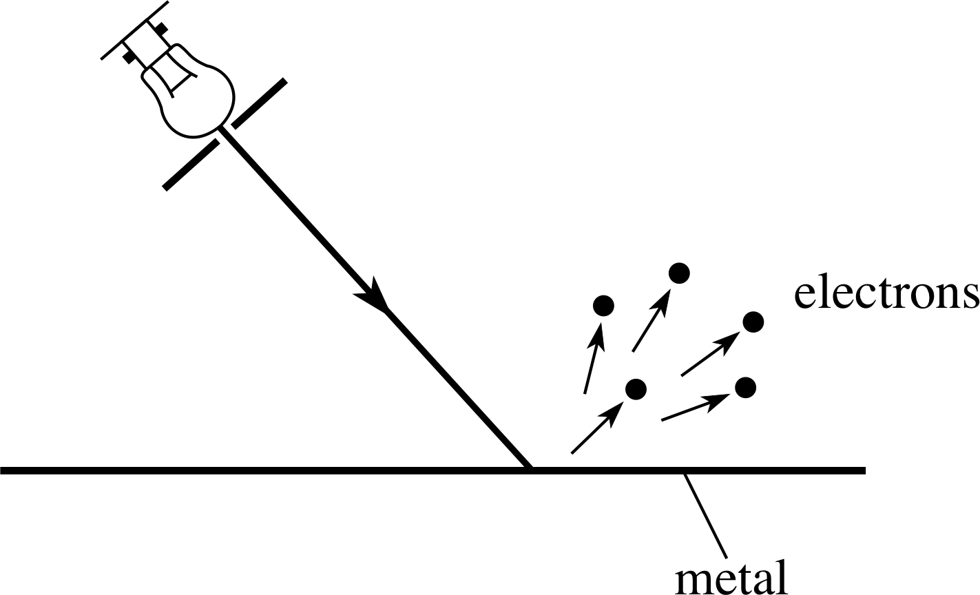
Figure 1 When electromagnetic radiation (of sufficiently high frequency) impinges on the surface of a metal, electrons are ejected. This is the photoelectric effect.
It is well known that energy is carried by radiation, as the warmth of sunlight amply demonstrates. In this section we consider how radiation transfers energy when it interacts with a surface. In particular, we will be concerned to study how the electrons in a metal surface absorb the energy.
2.1 Observation of the photoelectric effect
Soon after the discovery of the electron it was found that they could be produced by shining ultraviolet radiation on to a metal surface. This effect, the photoelectric effect, was examined carefully by the German physicist Philipp Lenard (1862–1947) between 1886 and 1900; he found that in any particular experiment these photoelectrons were emitted from the surface (Figure 1) with a range of kinetic energies up to some maximum value.
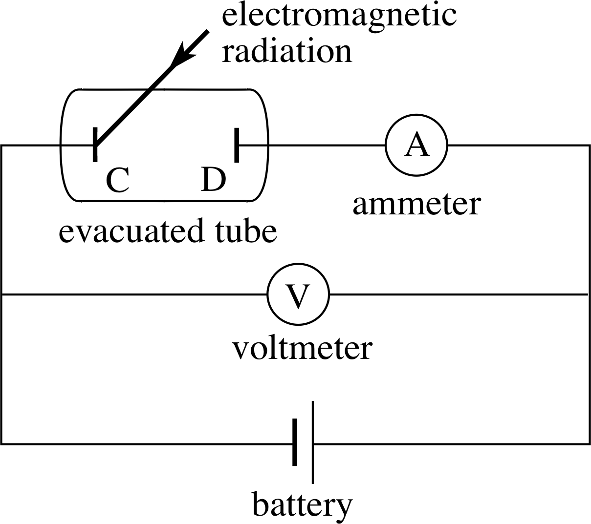
Figure 2 A circuit diagram of the apparatus for investigating the photoelectric effect. C and D are metal plates enclosed in a vacuum tube, and the light shines on to plate C.
The analysis of this simple result had far reaching consequences for our understanding of the nature of light. Albert Einstein (1879–1955) eventually showed that the photoelectric effect provided direct evidence that the model of light as an electromagnetic wave was inadequate. Even earlier evidence of this inadequacy had arisen from the observed spectrum of light emitted by a hot object, the so–called spectrum of black-body radiation, but this evidence was more indirect and more difficult to appreciate so we will delay discussion of it until Subsection 5.1. i
First then, let us see what sort of apparatus is needed for the investigation of the photoelectric effect. Figure 2 shows schematically how the experiment is done. The plates C and D in the evacuated tube are the central part of the apparatus. Plate C is illuminated by the light source, and the electrons emitted are collected by the plate D. If plate D is at a positive potential with respect to plate C, as in Figure 2, and if this potential difference is not too close to zero, then all the electrons emitted will be attracted by plate D and the electric current generated is independent of the battery voltage.
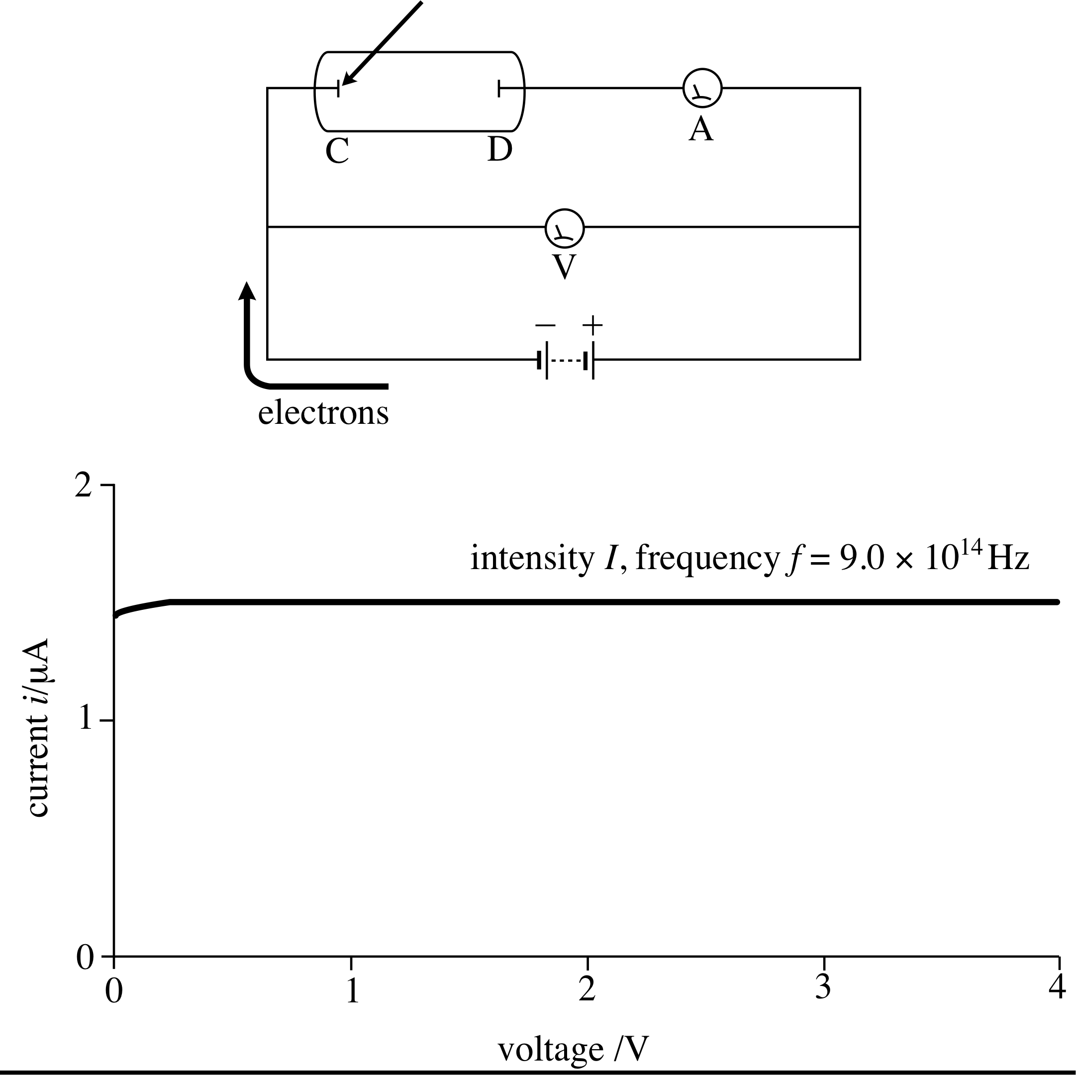
Figure 3 Plate D is at a positive potential V with respect to plate C, so all electrons ejected from plate C are attracted to D. The rate of flow of electrons, and so the current, does not depend on the voltage of plate D, provided this voltage is not too close to zero.
This is illustrated in Figure 3, where the plate is illuminated by ultraviolet light.
Question T1
If an electron leaves the metal surface at a speed υ, what will be its kinetic energy when it arrives at plate D, if the voltage difference is V?
Answer T1
The initial kinetic energy of the electron is $\frac12m\upsilon^2$. It is attracted, and so accelerated, by plate D, so its final kinetic energy is $\frac12m\upsilon^2 + eV$, where e is the magnitude of the charge on the electron.
We will use this result later.
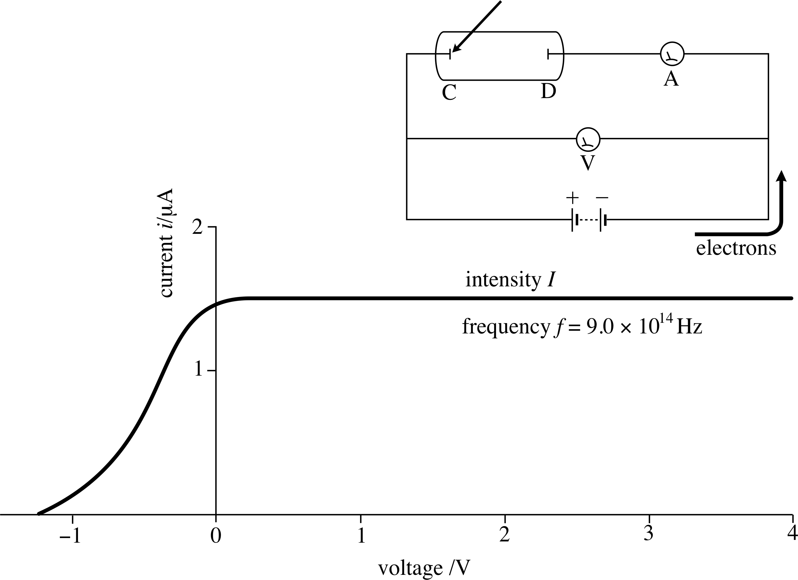
Figure 4 Plate D is at a negative potential with respect to plate C, so that electrons from plate C are repelled, and only the more energetic ones are able to reach plate D.
If we now reverse the battery terminals, so that plate D becomes the negative plate, as in Figure 4, then the electrons will be subject to a repulsive force. An electron emitted with kinetic energy $\frac12m_{\rm e}\upsilon^2$ will be slowed down or even stopped by the electric field, if the field is strong enough.
An electron arriving at D will then have a reduced kinetic energy $\frac12m_{\rm e}\upsilon^2-e\lvert V\rvert$, where the positive quantity $\lvert V\rvert$ represents the magnitude of the (negative) voltage V. Thus, only those electrons with initial kinetic energy greater than $e\lvert V\rvert$ will reach plate D and contribute to the current, as the graph in Figure 4 shows.
The current produced gradually decreases as V becomes more and more negative, and finally, when the magnitude Vs of the voltage is just enough to stop the most energetic electrons (with speed υmax) from reaching the plate, we have
$\frac12m_{\rm e}\upsilon^2 = eV_{\rm s}$(1)
This voltage Vs is called the stopping voltage and gives a measure of the maximum kinetic energy for the electrons emitted from the surface.
It is not surprising that the electrons are emitted with a range of kinetic energies up to a certain maximum. Some energy is needed to extract electrons bound in the metal, and we would not expect them all to be bound with exactly the same energy. The electrons emitted with the highest energy presumably are those which are bound least securely and the range of kinetic energies comes from the range of binding energies in the metal.
According to the wave model of light the rate of energy transport in a light wave is determined only by its intensity and this is proportional to the square of the amplitude of the wave. i
✦ What does the wave model predict would happen to the current and the maximum kinetic energy in the photoelectric effect if the intensity of the light falling on the surface is increased?
✧ If the electrons receive more energy per second we might expect that both the rate of electron emission (i.e. the current) and their maximum kinetic energy would be increased.
When this experiment was performed it was found that the electron current did indeed increase in proportion to the light intensity, but the maximum kinetic energy remained unchanged! This astonishing result was completely at variance with what was expected from the known physics of the day.
With the light source that Lenard used (an arc lamp), he was not able to say much more, except that the maximum electron kinetic energy was greater if blue light rather than red light was used. In other words, the maximum electron kinetic energy increased with the frequency of the light but not with its intensity. This happened for all the metals that he tried, so the result was quite general. Thus a new explanation for the interaction of the light with the metal was needed. This explanation would have to be radically different from the standard theory of electromagnetic waves, which had been so successful in accounting for the interference and diffraction of light.
2.2 A photon model for the light interaction: Einstein’s theory
An explanation of the photoelectric effect was provided quite quickly by Einstein, in 1905, based on the same idea that Max Planck (1858–1947) had introduced in 1900, to account for the spectrum of black–body radiation. (Subsection 5.1 discusses the topic of black–body radiation.) Planck had found that it was necessary to assume that electromagnetic radiation of frequency f could only be emitted or absorbed in finite amounts of energy, or packets; these came to be called quanta (singular, quantum). The amount of energy E in each quantum was proportional to the frequency f of the light, through the relationship:
Planck–Einstein formula: E = hf(2)
Equation 2 is now called the Planck–Einstein formula. h is a constant known as Planck’s constant, the value of which is now known to be approximately 6.626 × 10⁻³⁴ J s. These quanta of radiation later came to be called photons. In fact a photon is more than just a certain quantity of energy of radiation; it behaves as a genuine particle, having energy, momentum and a direction of motion. Although we have not yet presented the evidence for this, it is convenient to start using the word photon now.
Einstein suggested that each photon was completely absorbed by a single electron in the metal; its energy might then be enough to release the electron from the metal. The principle of conservation of energy allows us to represent the energy exchanges in this picture of the photoelectric effect as follows:
$\left(\large\substack{\text{energy of}\\[2pt]\text{incident}\\[3pt]\text{photon}}\right) - \left(\large\substack{\text{energy required to}\\[2pt]\text{remove electron}\\[3pt] \text{from metal}}\right) = \left(\large\substack{\text{kinetic energy}\\[2pt]\text{of outgoing}\\[2pt] \text{electron}}\right)$
If we restrict our attention to the maximum electron kinetic energy arising from absorption by those electrons with the minimum binding energy in the surface we have:
$\left(\large\substack{\text{energy of}\\[2pt]\text{incident}\\[3pt]\text{photon}}\right) - \left(\large\substack{minimum\text{ energy}\\[2pt]\text{required to remove}\\[3pt] \text{electron from metal}}\right) = \left(\large\substack{maximum\text{ kinetic}\\[3pt]\text{energy of}\\[2pt] \text{outgoing electron}}\right)$
We can express this as Einstein’s photoelectric equation:
Einstein’s photoelectric equation: $hf - \phi = \frac12m_{\rm e}\upsilon_{\rm max}^2$(3)
ϕ is a constant for a given metal, known as the work function of the metal. It is the minimum binding energy, or the minimum energy needed to remove an electron from the surface. Let us see how Equation 3, with its implication that each photon is absorbed by a single electron, explains the four main features of the photoelectric effect:
- 1
-
the maximum electron energy i does not depend on the intensity of the incident radiation;
- 2
-
the maximum electron energy depends on the frequency of the incident radiation;
- 3
-
there is a threshold frequency for a given metal; if light of a lower frequency than this is used then no electrons will be emitted, however intense the light;
- 4
-
once the frequency is above the threshold value, the electron current is proportional to the light intensity but there is no time delay in the emission of electrons, however low the intensity of the light.
Equation 3 shows us straightaway that the maximum energy depends only on frequency; this disposes of points 1 and 2 above. For point 3 we only need to note that if hf < ϕ then no electron can be ejected, since not enough energy can be supplied by any single photon. As regards point 4 above, once photons of sufficient energy become available the electrons can immediately begin the absorption and a single absorption is sufficient to cause an electron to be emitted, with no time delay required. In addition, the number of electrons emitted will be proportional to the number of photons arriving; this is why the electron current is proportional to the intensity once the threshold frequency has been exceeded.
✦ What do you suppose happens to the energy of the photon when the absorbed energy is insufficient to allow the electron to escape?
✧ The electron must gain energy but since it is unable to escape it will then eventually lose this energy through collisions with the crystal lattice. The energy then appears as thermal energy and the surface warms slightly.
Equation 3 also provides what every good scientific theory should provide, a testable prediction. It predicts a straight–line relation between the maximum electron kinetic energy and the frequency of the radiation. This prediction is easy to test. To do this it is necessary to find the maximum electron kinetic energy for a range of frequencies.
The maximum electron kinetic energy for any frequency can be found by measuring the stopping voltage for that frequency. Combining Equation 1,
$\frac12m_{\rm e}\upsilon^2 = eV_{\rm s}$(1)
and Equation 3 we have:
hf − ϕ = eVs(4)
i.e.Vs = (h/e)f − ϕ/e(5)
Equation 5 predicts that if Vs is plotted against the frequency f we should find that the points lie on a straight line. The intercept on the voltage axis is (−ϕ/e) which depends on the target, but, irrespective of the target, the line should have gradient (h/e). Thus, a graph of Vs against f should allow both Planck’s constant h and the work function ϕ for the target metal to be measured.
Many such investigations were conducted by Robert Millikan (1868–1953), in a series of very careful experiments carried out over several years and completed in 1916. Millikan confirmed Einstein’s predictions, and the value he obtained for h was in good agreement with values found by other methods. It is interesting to note that Millikan was rather reluctant to accept this result. Many years later he wrote:
I spent ten years of my life testing that 1905 equation of Einstein’s and contrary to all my expectations I was compelled in 1915 to assert its unambiguous verification in spite of its unreasonableness, since it seemed to violate everything we knew about the interference of light.
(Reviews of Modern Physics 21, 343, 1949)
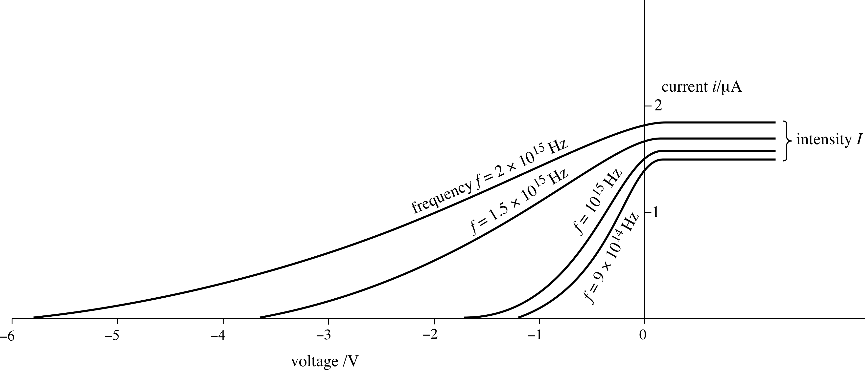
Figure 5 The effect on the graph of Figure 4 of increasing the frequency f of the radiation, with the intensity held constant.
The sort of results that are found experimentally are shown in Figure 5, which shows the effect of increasing the frequency of the light, with the intensity held constant.
At any particular light frequency we can see that the current flowing depends on the voltage applied; the stopping voltage at this frequency is the magnitude of the voltage at which the current falls to zero.
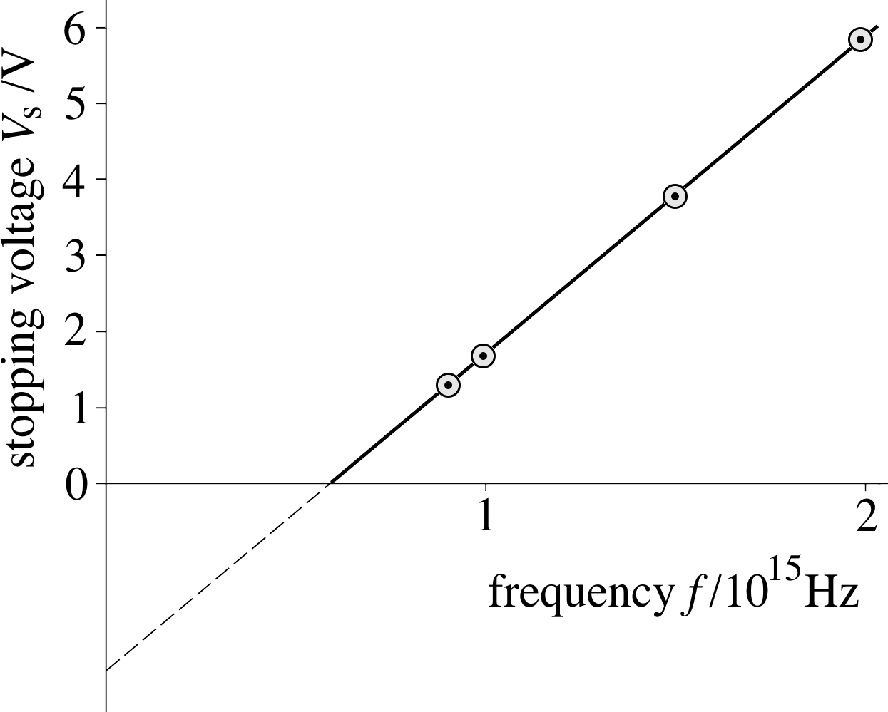
Figure 6 The variation of the stopping voltage Vs with the frequency of the radiation incident on the plate C.
If we repeat this measurement for a series of different frequencies we can plot a graph, such as that shown in Figure 6. The data in this figure are taken from the graph shown in Figure 5 – check for yourself that this has been done correctly.
Millikan was in good company. Very few people accepted Einstein’s picture of individual packets of radiation; in fact Einstein himself was so cautious about pushing the idea that his colleagues were often under the impression that he had given it up! The evidence for the wave model, coming from interference and diffraction, was so strong that it was very hard to abandon it. However, everything that came later confirmed the ‘unreasonableness’ of Einstein’s proposal.
It is instructive to consider further the time scale for the emission of electrons in the photoelectric effect, since this highlights the difference between the wave and photon models. The photoelectric process is not very efficient: several hundred photons are absorbed for each electron emitted from the surface. Nevertheless, it is found experimentally that electrons are emitted from the metal almost instantaneously (within a nanosecond, 10−9 s) once the light is switched on, however weak the source of light. With a weak source of light one might expect, on the basis of the wave model, that it would take several minutes to accumulate enough energy at the site of a particular atom to eject an electron, but this is not the case.
Question T2
(a) A light source emits light of high enough frequency to eject electrons from a potassium target 1 m away. If the source emits light at a rate of 8.0 W, the classical wave model predicts that this will spread uniformly around the source. If the radius of a potassium atom is 5.0 × 10⁻¹¹ m, at what rate does energy arrive at an atom in the target, according to the wave model?
(b) If the work function for potassium is 3.4 × 10⁻¹⁹ J, how long would it take an atom to acquire enough energy to emit an electron, according to the classical wave model of light?
Answer T2
(a) At 1 m distance we can expect the light to be spread uniformly over the surface of a sphere: a total area of 4π m2. The target area of a potassium atom will be π × (5.0 × 10⁻¹¹)2 m2, so that the power reaching one atom is:
(8.0 W/4π m2) × π × (5.0 × 10⁻¹¹ m)2 = 5.0 × 10⁻²¹ W
(b) The minimum time is the work function divided by the power:
3.4 × 10⁻¹⁹ J/5.0 × 10−21 W = 68 s
Since electrons are emitted within 10−9 s of switching on the light, the classical wave model is plainly inadequate.
There remains one problem about all this which may be worrying you. You may be wondering why an electron is unable to accumulate several photons, rather than only one, before attempting to leave the surface. Such a possibility would deny the existence of any threshold frequency since multiple photon absorptions would then allow any electron to accumulate sufficient energy to escape with any frequency of incident light, given sufficient numbers of photons.
✦ Think for a moment about this: can you suggest any reason why these multiple photon absorptions did not happen in Millikan’s experiments?
✧ The explanation lies in the time scale for the process, as discussed above. Once a single photon is absorbed, the electron will either escape (if possible) or lose its energy, within a nanosecond, through collisions with the metal target. If it is to absorb another photon before the earlier energy is lost within the target then it must do so in a time less than this. With the light sources available then, the probability of this was negligibly small. i
2.3 Radiation emitted by an accelerated charge and X–ray emission
If an energetic electron hits a target, such as the target of an X–ray tube, some or all of its energy is converted into electromagnetic radiation. This process converts the kinetic energy of the electron into energy of electromagnetic radiation. According to the classical theory of electromagnetic radiation this general process is expected whenever an electric charge is accelerated or decelerated, as in a collision. When the spectrum of this radiation is examined it is found that all frequencies are emitted up to some maximum value, which depends on the energy of the electrons hitting the target. This emitted radiation is known as bremsstrahlung (braking radiation).
Einstein’s equation, Equation 3,
$hf - \phi = \frac12m_{\rm e}\upsilon_{\rm max}^2$(Eqn 3)
provides a simple explanation of this process in terms of what amounts to an inverse photoelectric effect. As we have used Equation 3 so far it implies a conversion between photon energy and electron kinetic energy; the inverse process converts the electron kinetic energy into photon energy and photons are produced as the electrons slow down in the collision. A particular collision may produce a photon as well as some thermal energy in the target. Each time an electron of kinetic energy Ee loses energy by radiation, a photon of appropriate frequency must be produced to carry away this energy. All emission frequencies are possible up to some limit, fmax, which corresponds to the complete loss of the kinetic energy as radiation.
To represent this process we can rewrite Equation 3 in the modified form:
$hf_{\rm max} - \phi = \frac12m_{\rm e}\upsilon^2 = E_{\rm e}$
i.e.$f_{\rm max} = \dfrac{E_{\rm e}+\phi}{h} \approx \dfrac{E_{\rm e}}{h}$(6)
We have neglected the work function on the right of Equation 6 since work functions for most targets of interest are of the order of a few eV and significant intensities of emitted radiation only occur for incident electron energies of many keV, with emissions then in the X–ray region.
Figure 2 A circuit diagram of the apparatus for investigating the photoelectric effect. C and D are metal plates enclosed in a vacuum tube, and the light shines on to plate C.
2.4 Applications of the photoelectric effect
We have so far stressed the fundamental scientific importance of the photoelectric effect. There are also many practical applications of the process. Photoelectric cells of the sort used to demonstrate the photoelectric effect, and shown in Figure 2, are called photo-emissive cells, and were once used extensively for the measurement of light intensity.
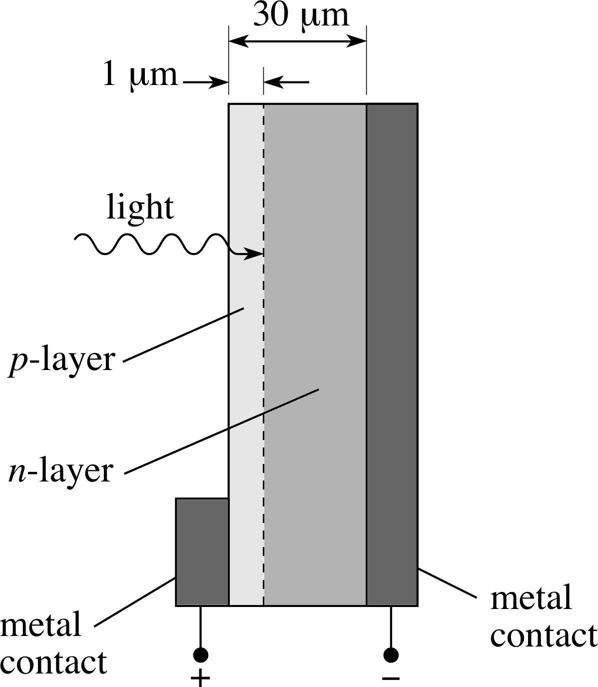
Figure 7 A silicon p–n junction photodiode, often arrayed to produce a solar cell. The diagram is not drawn to scale.
For most purposes today they have been superseded by semiconductor cells, such as the silicon p–n junction photodiode, illustrated in Figure 7. i Arrays of such cells are often used to make a solar cell, to convert solar light energy into electrical energy. The photodiode relies on the production of free charges in the material, following the absorption of light, but differs from photo–emissive cells in that the charges are not emitted from the material but remain within it, able to contribute to electrical conduction. These devices generate a voltage, even when irradiated by visible light. They are often used as power supplies in satellites, and are increasingly used as power supplies on Earth, for use in places where sunny weather can be relied upon where conventional power sources are not always available.
2.5 Summary of Section 2
The significant non–classical features about the photoelectric effect are that:
- 1
-
The maximum energy of the emitted electrons is given by Einstein’s photoelectric equation
$hf - \phi = \frac12m_{\rm e}\upsilon_{\rm max}^2$(Eqn 3)
so the maximum energy depends on the frequency but not the intensity.
- 2
-
There is a threshold frequency, below which no electrons are emitted, irrespective of intensity.
- 3
-
The electrons are emitted almost instantaneously, however weak the light source.
All these features are compatible with the idea that light of frequency f consists of photons that carry an amount of energy E = hf.
Figure 4 Plate D is at a negative potential with respect to plate C, so that electrons from plate C are repelled, and only the more energetic ones are able to reach plate D.
Question T3
When barium plates are used in the tube in Figure 4 and when the battery is replaced by a piece of wire, the minimum frequency of the radiation which enables electrons to be emitted is 6.1 × 10¹⁴ Hz.
(a) Calculate the work function of barium.
(b) Calculate the stopping voltage required to prevent the arrival of electrons at plate D, if the frequency of the incident radiation is 9.1 × 10¹⁴ Hz.
Answer T3
(a) Since the minimum (threshold) frequency is f1 = 6.1 × 10¹⁴ Hz, the minimum energy required to eject an electron from barium is
hf1 = 6.6 × 10⁻³⁴ J s × 6.1 × 10¹⁴ s−1 = 4.0 × 10⁻¹⁹ J = 2.5 eV
(b) From Equation 4, hf − ϕ = eVs, and from (a) ϕ = hf1.
HenceeVs = hf − hf1 = h (f − f1)
andVs = (h/e)(f − f1) = 1.2 V
Question T4
Look again at the graph in Figure 4.1Figure 4.
(a) What is the stopping voltage in this case?
(b) What would be the stopping voltage if the intensity were halved and the frequency of the incident radiation were held constant at 9.0 × 10¹⁴ Hz?
(c) What would be the stopping voltage required if the frequency of the incident radiation were reduced to 8.0 × 10¹⁴ Hz, with the original intensity of the incident radiation?
Answer T4
(a) About 1.25 V. Note that the stopping voltage is expressed as a positive number because it is defined to be the magnitude of the voltage between the plates to just prevent electrons ejected from plate C reaching D.
(b) About 1.25 V. This is the same as in (a), because the stopping voltage is independent of the intensity of the incident radiation.
Figure 6 The variation of the stopping voltage Vs with the frequency of the radiation incident on the plate C.
(c) About 0.9 V. The variation of the stopping voltage Vs with the frequency of the incident radiation f is given by Equation 5,
Vs = (h/e)f − ϕ/e(Eqn 5)
First, we need the work function of the metal:
ϕ = hf − eVs
ϕ = 6.63 × 10⁻³⁴ J s × 9.0 × 10¹⁴ s−1 − 1.60 × 10−19 C × 1.25 V
ϕ = 4.0 × 10⁻¹⁹ J = 4.0 × 10⁻¹⁹ J/1.60 × 10−19 J eV−1 = 2.5 eV
(You could have found the answer directly from Figure 6, as the work function is just the intercept of this straight line with the Vs–axis.)
Now Equation 5 can be used to find Vs when f = 8.0 × 10¹⁴ Hz:
Vs = (hf − ϕ)/e
Vs = (6.63 × 10⁻³⁴ J s × 8.0 × 10¹⁴ s−1 − 4.0 × 10⁻¹⁹ J)/1.6 × 10−19 C
Vs = 0.82 V
You can check that this agrees with Figure 6.
3 Momentum carried by radiation and radiation pressure
In Section 2 we took the experimental observation that light can transport energy (consistent with a classical wave model) and we showed that, at least in interactions with electrons in a surface, it was necessary to have the energy exchanges quantized in packets (photons). It was only when we studied the details of the photoelectric effect that this basic ‘graininess’ in the energy transfer became apparent.
In this section we will start from another experimental observation that light can exert forces and hence a pressure on a surface on which it falls (again consistent with a classical wave model). We know that the origin of the pressure in a gas lies in the collisions between the molecules and the walls of the vessel which contain it. These collisions transfer momentum from the gas molecules to the walls and in Newtonian physics we associate momentum changes with forces. For radiation there is often no container, but the presence of a force exerted by light when it shines on a surface leads us to the belief that light transports momentum as well as energy. If we could show that the momentum transferred by light is also in quantized amounts, then we would be encouraged into associating this also with the quantum called the photon; we would then be much more justified in thinking of the photon as a genuine particle, carrying energy and momentum and delivering or removing these in interactions with matter. We are going too fast here – first we need to demonstrate that momentum is carried by light and then show that the momentum transfers between light and matter are quantized. These are the tasks for this section and the next section.
3.1 Wave model for the momentum carried by light
Whilst the wave model derivation of the expression for the momentum carried by electromagnetic radiation lies beyond the scope of FLAP the results are simple to quote and to use. These are summarized as follows:
If the radiation transports a total energy E in a given time, then the total momentum transported in this time is of magnitude E/c, where c is the speed of light in a vacuum. This expression is independent of the frequency and is responsible for the forces and the pressures exerted by radiation.
✦ Show that the units of E/c are consistent with those of momentum.
✧ E/c has units J/(m s−1) = kg(m s−1)2/(m s−1) = kg m s−1, as for momentum.
If the radiation falls on to a surface and is wholly absorbed, the momentum transferred to the surface is of magnitude E/c; if the radiation falls perpendicularly on to the surface and is wholly reflected then the momentum transferred to the surface is 2E/c; if the radiation is reflected at an angle θ then the momentum transferred perpendicular to the surface is of magnitude (2E/c) cos θ. i
Question T5
Energy is produced by the Sun at a rate of 3.9 × 1026 W. Assuming that this radiation spreads out uniformly from the Sun show that the pressure due to absorption of this radiation at a distance of the Earth’s orbit, 1.5 × 10¹¹ m, is about 4.6 × 10⁻⁶ Pa. i
Answer T5
The energy produced must be spread uniformly over a sphere of radius 4πr2 at the distance of the Earth’s orbital radius. So the energy falling on unit area per second here is 3.9 × 1026 W/(4π × (1.5 × 1011 m)2).
The momentum transferred per unit area per second is of magnitude E/c, which is
3.9 × 1026 W/(4π × 3.0 × 108 m s−1 × (1.5 × 1011 m)2 = 4.6 × 10⁻⁶ N m−2
If this is absorbed by a body, then the magnitude of the perpendicular force per unit area, i.e. the pressure, is the momentum absorbed per square metre per second, i.e. p = 4.6 × 10⁻⁶ Pa.
This radiation pressure is very weak, which is why its effects are hardly ever observed directly. One situation where it is observed is in the tails of comets. When a comet approaches the Sun its tail generally points away from the Sun irrespective of the direction of motion of the comet itself. This is due to the effect of radiation pressure on the head of the comet, creating a dust and gas cloud by evaporation, and then pushing this cloud away from the Sun. You may be surprised at this if you had supposed that the tail of a comet always trails behind its head. In fact, the Sun emits streams of particles as well as light and these also exert forces on impact; comet tails respond to both these effects and can sometimes be seen to consist of two distinct components.
It has been suggested that radiation pressure could be used as a means of propelling a spacecraft without the use of any fuel, rather as a yacht uses the pressure of the wind on Earth.
Question T6
Using the results of Question T5 calculate the minimum sail area needed to give a space yacht of mass 1000 kg an acceleration of 1 m s−2 when at the Earth’s orbital distance from the Sun and with the radiation fully absorbed. Would there be sufficient energy in this radiation for the intrepid explorer to cook breakfast?
Answer T6
The maximum force (and hence minimum sail area) would come with the sail area set perpendicular to the radiation flow. The magnitude of this force is then the radiation pressure times the sail area: F = PA. This force gives the yacht of mass m an acceleration of magnitude a = F/m = PA/m and so the minimum sail area is:
Amin = ma/P = 1000 kg × 1 m s−2/4.6 × 10−6 N m−2 = 2.2 × 10⁸ m2 (≈15 km)2
This area is rather unwieldy, even under weightless conditions!
The solar power captured (energy per second) = c × (momentum per second) = c × F = c × PA.
The captured power is then 3 × 10⁸ m s−1 × 4.6 × 10−6 N m−2 × 2.2 × 108 m2 = 3.0 × 101100 W = 300 GW. Certainly, breakfast would not be a problem – in fact this power would pose a major cooling problem.
The yacht is equipped better as a power station than as a means of transport.
The answer to Question T6 shows that the energy carried by light will be much easier to detect than its momentum. For example, if the sail area of our yacht were to be equipped with photo–voltaic cells and the power produced were then transmitted back to Earth we would have a sizeable solar power station; serious suggestions have been made along these lines.
3.2 Laboratory demonstrations of the momentum carried by light
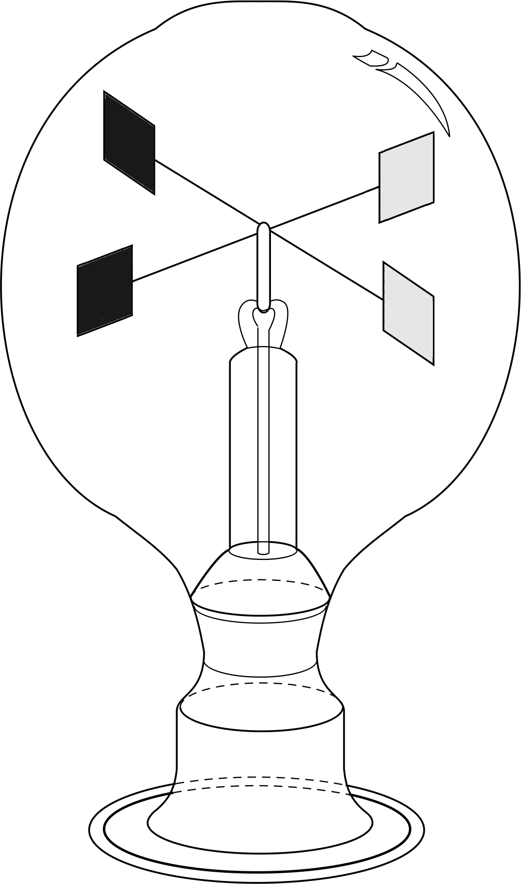
Figure 8a The Crookes radiometer. Each paddle is blackened on one face and made reflective on the other. Note that the paddles are in a vertical plane.
Coming down to earth, the existence of radiation pressure has been verified by sensitive laboratory experiments, and its magnitude has been shown to agree with the theory. A device which used to be seen regularly in optician’s windows, and may still be seen occasionally, is the Crookes radiometer (Figure 8a). This consists of a set of four vanes mounted on a pivot so as to form a sort of paddle-wheel, contained within an evacuated bulb. One face of each vane is blackened, the other is reflective.
✦ In Figure 8a, if light shines on to the vanes in the positions shown and with the light travelling into the page, in which sense should the vanes rotate due to radiation pressure?
✧ Since the light reflects back off the shiny surfaces but is absorbed by the blackened surfaces the pressure on the shiny surfaces is about twice as large and so the expected rotation is with the shiny surfaces pushed away from the incident light.
Unfortunately, when these devices are made the vanes almost always rotate the wrong way! The device rotates as expected if there is a very good vacuum in the bulb but any residual gases in the evacuated vessel will cause an opposite rotation. i
However, similar devices have been used successfully to show the radiation pressure effect. One such has a small rod suspended horizontally by a fine vertical fibre attached to its mid-point; a mirror is suspended from one end of the rod with a counterweight on the other end to keep the rod horizontal. When an intense beam of light (e.g. a laser) is reflected off the mirror the force on the mirror can be measured from the deflection of the suspension.
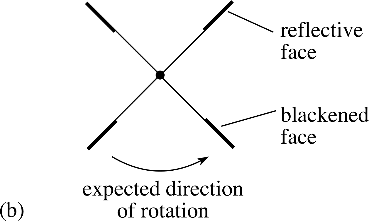
Figure 8b The Crookes radiometer. The expected sense of rotation of the vanes due to radiation pressure.
Although the existence of radiation pressure certainly implies the transfer of momentum by radiation, it does not imply the existence of photons as separate particles carrying momentum. However, if we were to find that the transferred momentum was quantized in definite amounts, then the idea of a photon as a particle would gain credibility.
Let us suppose for the moment that photons do exist as definite particles, so that a beam of light of frequency f takes the form of a stream of particles, each carrying energy E = hf and each having momentum of magnitude p (to be determined). In this simple model the total energy and momentum transferred over a period of time are obtained by multiplying the individual photon energies and momenta by the number of photons arriving over the period. The ratio of total energy to total momentum magnitude delivered by the beam must then be the same as the ratio of energy to momentum magnitude of an individual photon, since the number of photons involved cancels in the ratio.
✦ Use the expression for the ratio of energy to momentum transferred according to the wave model for light, together with the Planck–Einstein equation to predict the momentum magnitude p of an individual photon of energy E in a beam of wavelength λ.
✧ The result is simply p = E/c = hf/c = h/λ, where f is the frequency and λ is the wavelength of the associated radiation.
4 Photons as particles and the Compton effect
The photoelectric effect has given us a certain amount of new and unexpected information about the properties of light, but it raises quite a number of other questions. The most important of these is the nature of the packets in which radiation seems to be emitted and absorbed. If a packet of radiation is emitted, is it emitted in all directions, as the wave theory would suggest, or is it emitted in a form more like a particle? The fact that light is absorbed in packets and absorbed instantaneously suggests that it behaves more like a particle, but now we need direct evidence of photon momentum.
This evidence came from a crucial series of experiments, performed around 1920, that involved the scattering of X–rays by different targets. These experiments suggested that the scattered X–rays had a slightly longer wavelength (i.e. a lower frequency) than the incident radiation and also that the shift in wavelength depended on the scattering angle. These observations were inexplicable in terms of classical wave ideas. In the wave model the electrons in the target would be driven into oscillation by the oscillating electric field of the incoming electromagnetic wave. These oscillating electrons would then radiate as would any accelerated charge (see Subsection 2.3) and this would give rise to outgoing ‘scattered’ radiation. The wave model therefore predicts the same frequency for the scattered and incident radiations and certainly cannot explain any shift in the wavelength of the scattered radiation (or any radiation) with scattering angle.
An American physicist, Arthur H. Compton (1892–1962), gave a quantum interpretation of these experiments in 1922, about 20 years after the discovery and interpretation of the photoelectric effect. This scattering phenomenon later became known as the Compton effect. We will present Compton’s interpretation by assuming that photons exist as independent particles and then allow the success of the model in explaining the observations to justify this assumption. An underlying assumption in what follows will therefore be that the momentum magnitude p of a photon in a beam of light of wavelength λ is given by the relation deduced at the end of the last section:
photon momentum magnitude p = h/λ
4.1 Elastic collisions of photons and free electrons
The simplest way of showing that the photon can behave like a particle is to see whether it can undergo collisions like an ordinary particle, conserving energy and momentum in the collision and with the momentum transfers quantized, just like the energy transfers. To test this we consider the elastic collision of a photon with a free electron at rest. i We will see later that this situation can be realized by scattering X–rays or γ–rays from the electrons in matter.
We assume that a photon can undergo a particle–like collision, scattering through an angle θ, with the target electron recoiling so as to conserve energy and momentum. Immediately, we can appreciate that if some energy is transferred to the recoiling electron then the photon itself must lose this energy and so the scattered photon must have lower energy and a lower frequency (f = E/h) than the incident photon. Further, as for all particle–like collisions, the energy transfer will depend on the scattering angle and so the wavelength shift of the scattered radiation will depend on the scattering angle. Thus the quantum model correctly predicts (qualitatively) the two basic observations which had defeated classical physics!
To make these predictions quantitative we need to be able to write down the energy and the momentum of both participants and then apply the conservation laws for energy and momentum (components along and perpendicular to the direction of incidence). This will allow us to deduce a relationship between the initial and final energies of the photon and to relate this to the angle through which it is scattered in the collision. Finally we must compare this with experiment.
This strategy is fine, and we can use our deduced expressions for the energy and magnitude of momentum of a photon (E = hf, p = E/c = hf/c) but we run into a problem with the kinetic energy and the momentum of the scattered electron. The problem is that the scattered electron is likely to be travelling at a substantial fraction of the speed of light and the Newtonian expressions for momentum and kinetic energy break down and must be replaced by their relativistic equivalents.
The thing we need to know is the relationship between the momentum and the kinetic energy of the electron. For Newtonian mechanics, with me as the electron mass, pe = meυ and Ekin = meυ2/2 and so the relationship is:
Ekin = pe2/2me
The relativistic version of this, for the electron, is:
(Ekin + mec2)2 = (mec2)2 + (pec)2(7) i
where c is the speed of light in a vacuum.
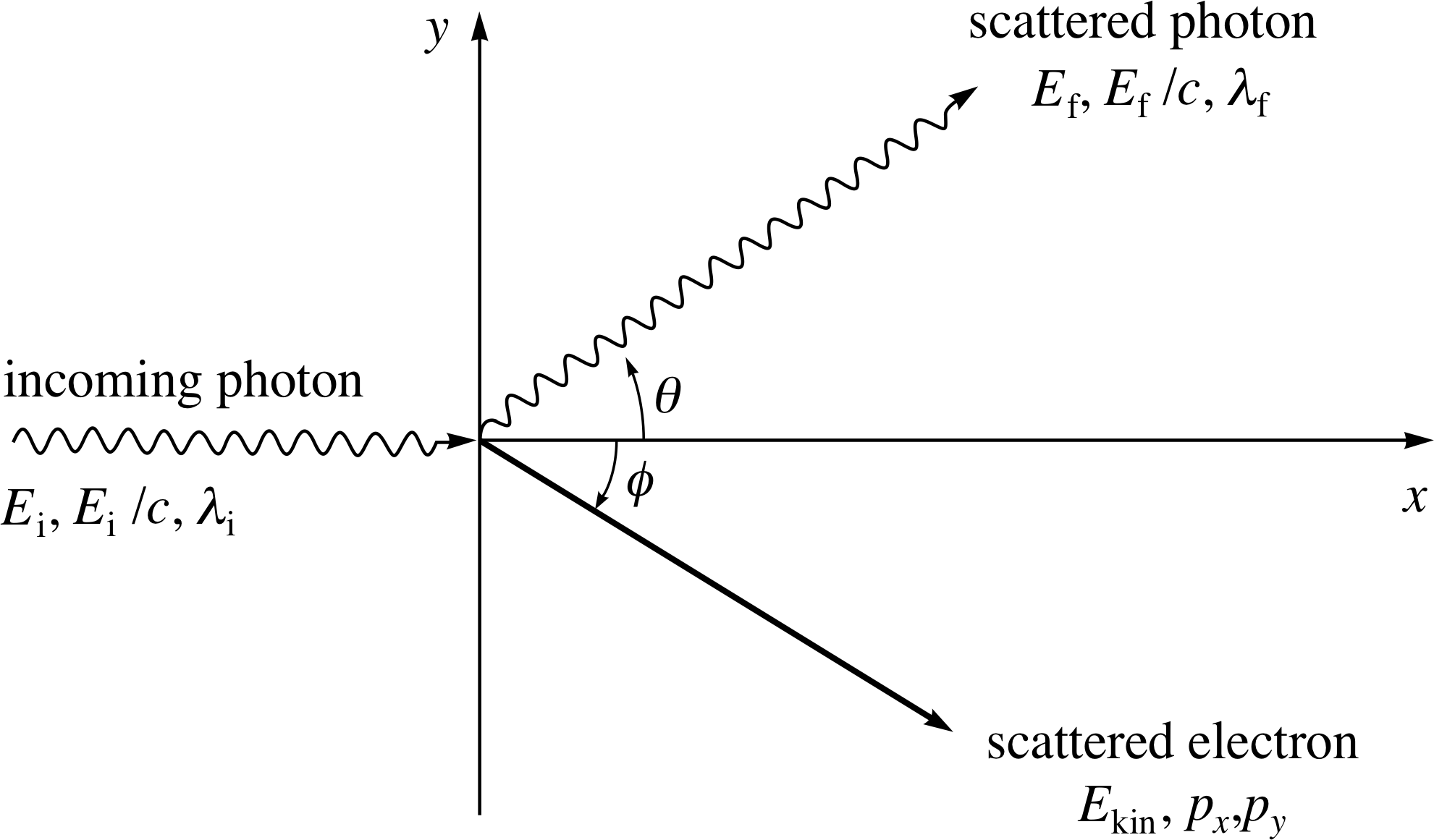
Figure 9 A schematic representation of Compton scattering, in which an incoming photon scatters from an electron at rest.
Consider the collision shown in Figure 9. A photon with initial energy Ei, momentum magnitude Ei/c and wavelength λi, moving along the x–axis, collides with an electron at rest and is scattered through an angle θ. After the collision the scattered photon has a final energy Ef, momentum magnitude Ef/c, and wavelength λf. The electron has kinetic energy Ekin and momentum components px and py after the collision.
We now treat the problem as we would any particle–particle collision and apply the conservation principles for energy and momentum (components along the x– and y–axes) before and after the collision:
energy:Ei = Ef + Ekin(8)
x–momentum:Ei/c = (Ef/c) cos θ + px(9)
y–momentum:0 = (Ef/c) sin θ + py(10)
We do not need to go through the algebra in detail, but if you wish you can follow through the steps outlined below:
- 1
-
Use Equations 9 and 10 to express px and py in terms of Ei and Ef.
- 2
-
Use pe2 = px2 + py2 to substitute in Equation 7, so eliminating the momentum.
- 3
-
Equation 7 then gives an expression for Ekin, which can be substituted into Equation 8.
- 4
-
This finally leads to the (comparatively) simple equation
$E_{\rm f} = \dfrac{E_{\rm i}}{1+\left(E_{\rm i}/m_{\rm e}c^2\right)\left(1-\cos\theta\right)}$(11)
which tells us how the final energy of the photon depends on the angle of scattering. If we look at radiation that has been scattered through a particular angle we should be able to check Equation 11 and thereby test the assumption that the photon behaves like a particle with p = E/c in this situation. i
4.2 Observation of the Compton effect
In order to test Equation 11 we must choose an initial photon energy Ei that will allow the right–hand side of the equation to vary substantially as the scattering angle is changed. This requires that the two terms in the denominator are of similar size, with Ei/mec2 chosen to be of the order one so that the second term varies from zero to one as θ varies from 0° to 90°; if Ei/mec2 is significantly smaller than one then the second term in the denominator will be swamped by the first.
Question T7
On this basis, what is an appropriate photon energy and the associated wavelength to show the Compton effect for electrons?
Answer T7
mec2 = 9.1 × 10−31 kg × (3.0 × 108 m s−1)2 22= 8.2 × 10⁻¹⁴ J = 0.51 × 10⁶ eV.
So for (Ei/mec2) ≈ 1 we must have Ei ≈ 8.2 × 10⁻¹⁴ J ≈ 0.51 MeV.
This corresponds to a frequency of Ei/h = mec2/h = 1.2 × 10²⁰ Hz
and a wavelength of c/(Ei/h) = h/mc = 2.4 × 10⁻¹² m.
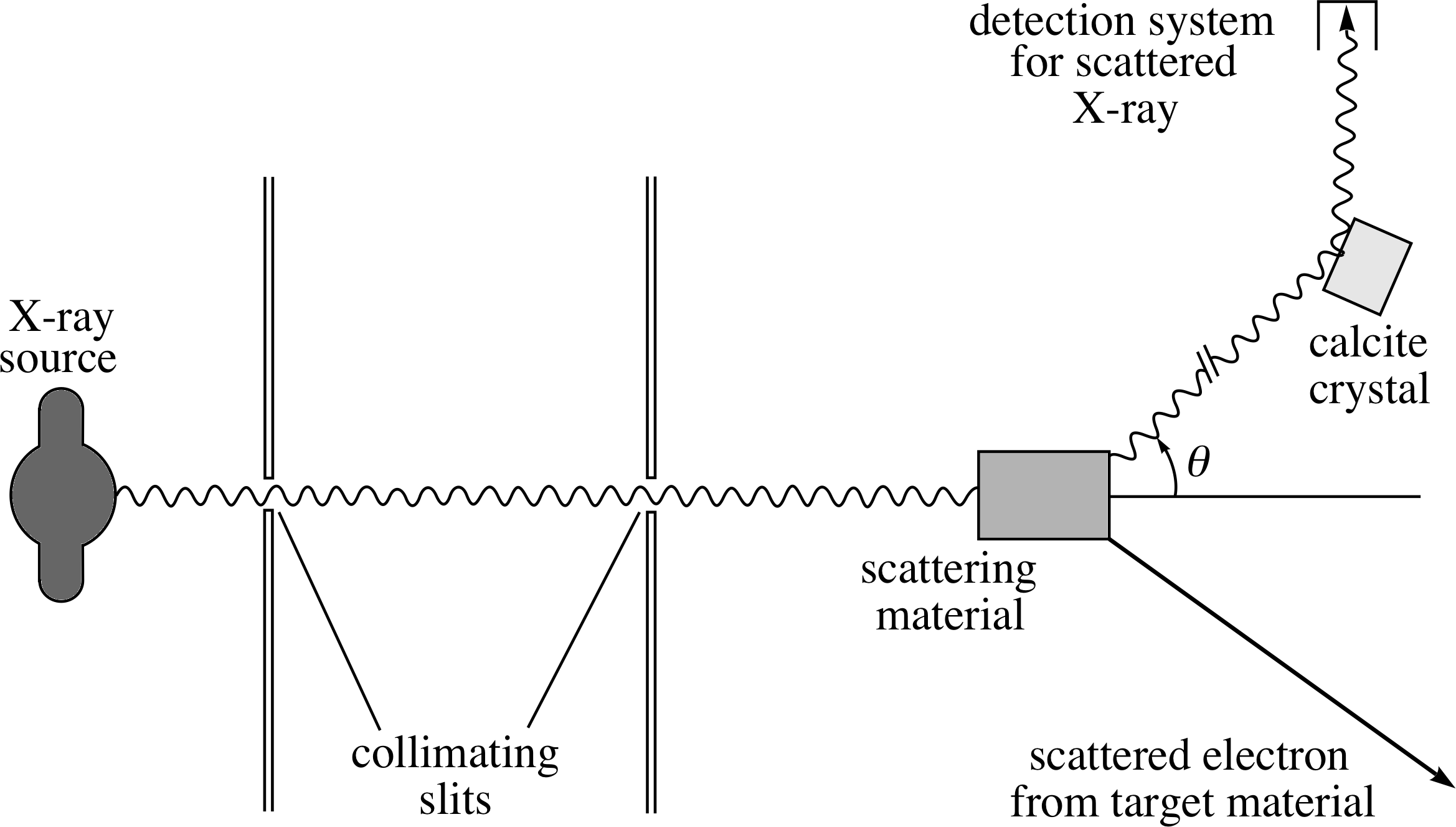
Figure 10 Compton’s scattering apparatus.
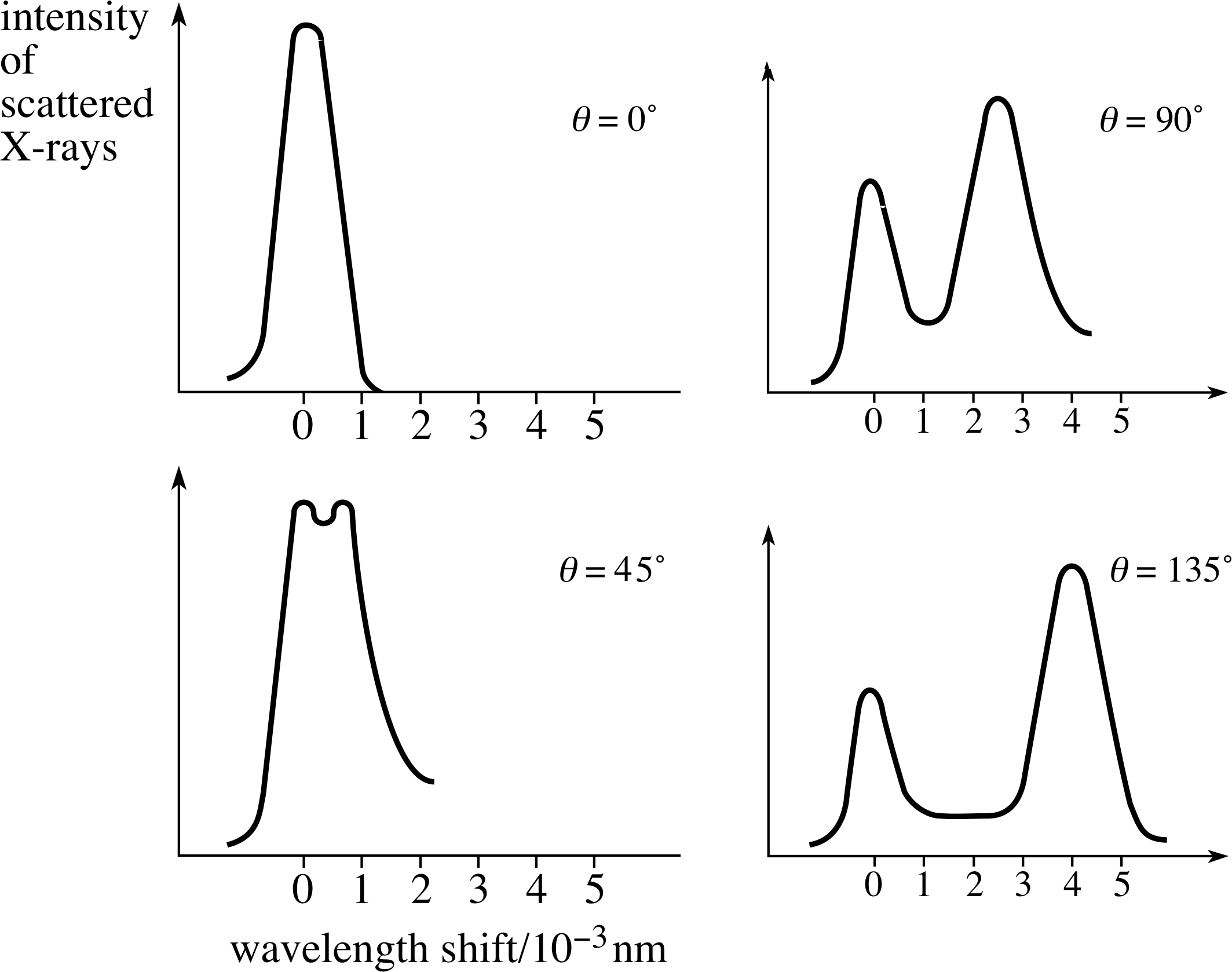
Figure 11 Results from a typical Compton scattering experiment.
This suggests that we should use radiation of wavelength 2.4 × 10⁻¹² m, or something not too much larger. The quantity (h/mec) is known as the Compton wavelength of the electron, and it is an important quantity whenever the interaction of an electron source with light is considered. Compton’s own experimental apparatus is shown schematically in Figure 10. X–rays from a molybdenum target and of wavelength 7 × 10⁻¹¹ m pass through a pair of collimating slits (which define the incident direction) and then collide with electrons in a solid material. i The wavelength of those X–rays which are scattered through an angle θ is measured by an interference method (a calcite crystal acting as a diffraction grating). This X–ray wavelength is very much longer than the ideal which we have just calculated, but Compton was limited by what could be produced at the time.
Figure 11 show a typical set of results for a Compton scattering experiment using X–rays of initial wavelength λi = 7.08 × 10⁻¹² m, scattered from a carbon target. The intensities of the scattered X–rays, which have a final wavelength λf, are plotted against their wavelength shift, λf − λi, for various scattering angles θ.
In the analysis of such experiments it is convenient to rewrite Equation 11,
$E_{\rm f} = \dfrac{E_{\rm i}}{1+\left(E_{\rm i}/m_{\rm e}c^2\right)\left(1-\cos\theta\right)}$(Eqn 11)
in terms of the initial and final wavelengths λi and λf.
Question T8
Use Equation 11 to show that, for Compton scattering:
λf − λi = (h/mec)(1 − cos θ)(12)
Answer T8
Since E = hf = hc/λ, we have from Equation 11,
$E_{\rm f} = \dfrac{E_{\rm i}}{1+\left(E_{\rm i}/m_{\rm e}c^2\right)\left(1-\cos\theta\right)}$(Eqn 11)
$hc/\lambda_{\rm f} = \dfrac{hc/\lambda_{\rm i}}{1+\left(hc/\lambda_{\rm i}/m_{\rm e}c^2\right)\left(1-\cos\theta\right)}$
Cancelling hc from both sides and turning it all upside down gives us:
λf = λi[1 + (hc/λimec2)(1 − cos θ)] = λi + (h/mec)(1 − cos θ)
i.e.λf − λi = (h/mec)(1 − cos θ)(Eqn 12)
We can see from Equation 12 that the experimental results obtained by Compton are in good agreement with the predictions of the particle model. i
In general, the experimental results of Compton scattering show the following features:
- 1
-
The scattered radiation consists of two wavelengths, the original one λi and an additional one λf. i
- 2
-
λf is always greater than or equal to λi.
- 3
-
λf depends on the scattering angle.
- 4
-
λf does not depend on the material of the target.
- 5
-
λf obeys the angular dependence predicted by Equation 12.
In a later experiment Compton confirmed the particle model further by showing that the recoiling electron had the energy and direction expected. Walther Bothe (1891–1957) and Hans Geiger (1882–1945) showed that the scattered photon and electron appeared at the same time. Thus, almost everything that could be required of a particle seemed to have been demonstrated. However awkward it might be, it seemed to be certain that the photon behaved as a particle.
4.3 Some further questions concerning the Compton effect
In our discussions of the Compton effect so far we have presented the main issues, without complication, but this means that we have glossed over a few subtleties, some of which may already have occurred to you and may even be concerning you. We can now raise these issues through a series of questions.
Study comment Some of the issues raised here are not simple so you should not worry if you find them difficult; the questions are related to each other and should be considered in the sequence given. You may wish to consider them for a while before you read the answers. If your situation allows it, you could discuss these questions with other students first.
✦ Our model has treated the electrons as free particles yet in the experiments we have used electrons which were either bound in atoms or in a material. Is it valid to treat them as free particles?
✧ For photons of several hundred keV, such as we are using, the binding energies of electrons either to atoms or within materials (e.g. work functions) are insignificant and we can consider them to be free.
✦ What would be the effect if the photons were scattered not from free electrons but from electrons which remained bound in an atom?
✧ If the scattered electron remained in the atom then the whole atom would recoil and the effective mass to be used in Equation 12,
λf − λi = (h/mec)(1 − cos θ)
would be the atomic mass, which is several thousand times greater than that for the electron. Equation 12 then predicts a negligible shift of wavelength.
✦ Can you explain the origin of the Compton scattered radiation which has the same frequency as the incident radiation (see Figure 11)?
✧ Any scattered radiation having the original wavelength must imply that the Compton shift in wavelength is negligible, such as when scattering from a particle of much higher mass than the electron. This can occur if the target electron remains within the atom and might be expected if the target electron were bound more tightly to the atom or the photon energy were not too large.
✦ Our model has treated the electrons as being at rest yet in the experiments we have used electrons in atoms and in materials and these electrons are not at rest. Is this valid and what effect might it have?
✧ Compared to the approaching photon, an electron must still be moving fairly slowly, so the approximation is not unreasonable. However, the effect would tend to make the correlation between scattering angle and energy loss rather less well–defined and so the observed peaks would be spread in wavelength; you can see this in Figure 11b where the Compton–shifted peaks are rather broader than the unshifted peaks.
✦ The Compton effect is not observed when visible light photons scatter from the electrons in a material; if it were we would find, for example, that when blue light scattered from a surface we would observe the scattered light as green or yellow or red, depending on the scattering angle! Why is Compton scattering only seen with X–rays or γ–rays?
✧ Photons of visible light have energies of only about 2 eV and so are very unlikely to knock the electrons from the atoms or the material. As discussed earlier this leads to a negligible shift of wavelength.
4.4 Summary of Section 4
The Compton effect has taken our knowledge of the photon one stage further; we can now be certain that there are some aspects of light that can only be explained by treating it as being composed of entities (photons), which behave like particles with a definite energy, momentum, and direction of motion.
Question T9
The qualitative features of Compton’s results are summarized in the box below.
- 1
-
The scattered radiation consists of two wavelengths, the original one λi and an additional one λf.
- 2
-
λf is always greater than or equal to λi.
- 3
-
λf depends on the scattering angle.
- 4
-
λf does not depend on the material of the target.
- 5
-
λf obeys the angular dependence predicted by Equation 12,
λf − λi = (h/mec)(1 − cos θ)(Eqn 12)
Explain briefly, in your own words, how each of these five characteristics can be accounted for using the photon model.
Answer T9
Characteristic 1 The scattered peak at longer wavelength corresponds to the photons transferring part of their energy to the recoiling electron and hence losing this energy themselves. The scattered peak at the same wavelength corresponds to the photons scattering from tightly bound electrons which remain within their respective atoms after the collision. Since the atom as a whole recoils, the mass difference between the two participants is such that the photon scatters elastically with essentially unchanged energy.
Characteristic 2 This is implied by Equation 12,
λf − λi = (h/mec)(1 − cos θ)(Eqn 12)
since (1 − cos θ) cannot be negative; it varies from 0, when θ = 0°, to 2, when θ = 180°. Also the photon can only lose energy when it scatters from a stationary electron.
Characteristic 3 This is implied by Equation 12, which shows that λf depends on cos θ.
Characteristic 4 This is implied by Equation 12, since none of the quantities in the equation depend on the nature of the target, only that free electrons are involved. At these photon energies all materials can be considered to contain free electrons.
Characteristic 5 This simply states that the particle model, leading to Equation 12, is supported by the experimental evidence.
5 More about photons
In this section we describe some other experiments which either consolidate our view of the photon as a particle or show further aspects of its behaviour.
5.1 Black–body radiation
From the historical perspective this subsection should have begun our module. Planck’s investigation (1900–) of the wavelength distribution of the light emitted by an ‘idealized’ hot body, the so–called black-body spectrum, provided the first evidence that the interactions of radiation with matter were quantized. A full understanding of this theory requires quite a lot of mathematics, and this module is not the place to go into this; however, the basic points of the argument can be appreciated without much complexity and this will be our approach here.
Any body will generally both absorb and emit radiation. If the temperature of the body is sufficiently high, the emitted radiation may be visible and the body may be seen to glow, but even if this is not the case, emission still takes place.
When the radiation from a body is examined it is often found to contain all possible wavelengths within a wide continuous band; when this is the case the body concerned is said to have a continuous_spectrum_emission_or_absorptioncontinuous emission spectrum. i The Sun is an example of such a body; the white light that it produces contains all the colours of the rainbow.
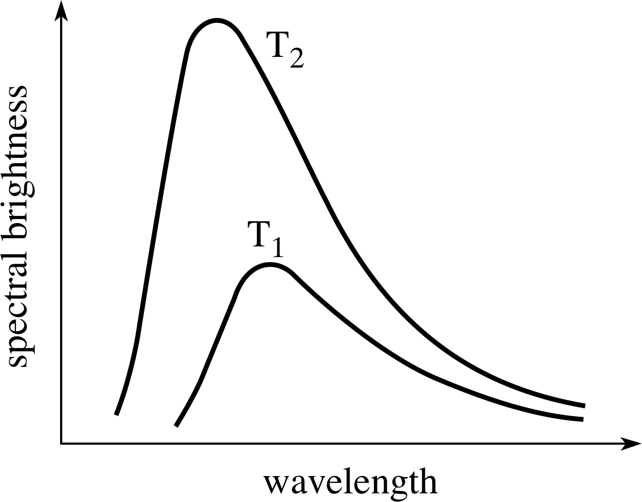
Figure 12 The continuous emission spectrum from an idealized hot body, the so–called black–body radiation. The vertical scale shows the spectral brightness of the surface and the horizontal scale shows the wavelength. The spectrum from the same body at two different temperatures (T2 > T1) is shown. Note that the peak of the spectrum shifts to shorter wavelengths as the temperature is increased.
The continuous emission spectrum of a body may be displayed graphically by plotting the relative brightness of unit area of the body’s surface against the wavelength at which it is observed. Such plots depend on the nature of the body as well as its temperature, but they always approximate to a greater or lesser extent an ideal emission spectrum that depends only on temperature. Two members of this family of ideal spectra, corresponding to different temperatures T1 and T2, are shown in Figure 12.
These ‘ideal’ emission spectra are often described as black–body spectra, since it can be shown that a perfect emitter of radiation will also be a perfect absorber (reflecting none of the radiation that falls upon it) and would therefore appear to be black were it not for its emissions. Of course, black bodies of this kind will not necessarily appear black at all. The Sun for instance, over a wide range of wavelengths, provides a good approximation to a black body with a temperature of about 5800 K, and it certainly does not look black!
A very close approximation to a black body can be produced in practice by cutting a small hole in a hot hollow body of uniform temperature, and observing the radiation coming from that hole. Since the hole is unlikely to reflect any of the radiation that falls upon it, it is almost perfectly black, and the spectrum of the emitted radiation will be almost entirely determined by the temperature within the cavity.
An explanation for the detailed shape of the black–body spectrum proved impossible in terms of classical physics. When electromagnetic wave theory was used to analyse the energy stored within a hot cavity, it was necessary to take into account all possible standing waves that might exist between the walls, for each possible wave frequency from zero to infinity. Classically, each of these possible oscillations contributes the same average energy to the cavity.
It was an embarrassing conclusion of this analysis that as higher frequencies are considered there are more and more possible standing waves per unit frequency interval and therefore a higher and higher energy density in the cavity.
The inescapable conclusion was that the total energy within the cavity should be infinite and the spectrum emitted from the black body should increase without limit at high frequencies – as if the long wavelength part of the curve in Figure 12 continued to rise as wavelength increased, rather than peaking and then falling back to zero again as experiment showed. This impressive failure of classical physics became known as the ‘ultraviolet catastrophe’! i
Planck took a different model, a quantum model. He assumed that the interaction between the radiation and the cavity walls involved quanta of energy, in emission and absorption. Specifically, he assumed that the walls contained oscillators and that an oscillator of frequency f cannot have any arbitrary energy but had energy_levelenergy states which were integral multiples of the product of a constant h and the oscillator frequency f. i
As the wall oscillators interact with the radiation in the cavity, each oscillator of frequency f can then only change its energy by multiples of hf. On statistical grounds, the higher energy states of an oscillator are less probable than the lower states and this discrimination means that the average energy associated with radiation at frequency f (wavelength λ) falls with decreasing λ (unlike in the classical model, where this is a constant, set by the temperature). If this average energy is then combined with the greater number of possible oscillators associated with decreasing λ (as for the classical model) we reach a prediction for the power per unit area (spectral brightness) in the cavity as a function of λ. This expression is known as Planck’s function. The detailed form of Planck’s function is not important for our purposes here but it is given in the marginal note, just for interest. i
When Planck’s result is compared with the observed black–body spectrum the agreement is excellent, providing the constant h is chosen appropriately. This success demonstrated that the energy states of an oscillator were quantized, not continuously variable as in classical physics, and that when radiation interacts with matter it does so by exchanging packets of energy or quanta.
This demonstrates the energy quantum of interaction but does not yet show the photon as a distinct particle. It is likely that Planck himself did not fully appreciate the impact these ideas were to have in the development of physics.
5.2 The ‘size’ of a photon
A wave, even a very weak one, is always spread out over a region of space and often continues for a considerable length of time – properties which cannot easily be reconciled with the picture of a particle.
For this reason, attempts were made to find out how large a target needed to be before the photoelectric effect could be observed; this would set an upper limit to the size of a photon as a particle. It has been found that metal particles as small as 10−7 m in diameter still show the effect with X–rays, which have a wavelength not much smaller.
It has also been shown that a photon can pass through a specially designed shutter in less than 10−9 s and light pulses shorter than 10−13 s can be produced from a laser, so the maximum length of a single photon in the direction of motion is less than 3 × 10⁸ m s−1 × 10⁻¹³ s = 0.03 mm i.e. 30 μm.
These limits are not measurements of the size of a photon but are simply experimentally determined upper bounds to a region of space within which a photon may be found. It could, in future, be discovered that a photon can be found within a region much smaller than this (about 60 wavelengths of light), but already these limits are a long way from what one would expect of an extended wave, and encourage one further to think that a photon is a particle. Nevertheless, most physicists are uneasy with the idea that a photon has a ‘size’ and usually try to avoid thinking in such terms.
5.3 Counting photons
As we saw in Section 2.2, the amount of energy contained in a single photon is extremely small, and so it is rather difficult to observe directly. For example, a 10% efficient 100 W light bulb emits about 3 × 10¹⁹ photons every second! In order to observe a single photon, we have to amplify its effects considerably. The human eye is remarkably good at detecting photons, as can be seen from the next question.
Question T10
On a dark night the human eye can just see the light bulb mentioned above at a distance of about 80 km. Use the data above to estimate the photon sensitivity of the eye (i.e. the minimum detectable number of photons per second), assuming the bulb radiates uniformly in all directions and that the diameter of the eye pupil is 5 mm.
Answer T10
If the bulb radiates 3 × 10¹⁹ photons every second and it does this uniformly over the surface area of a sphere of radius 8 × 10⁴ m then the rate of arrival at the eye pupil of area π × (2.5 × 10⁻³ m)2 is:
$\rm 3\times10^{19}s^{-1} = \dfrac{\pi(2.5\times10^{-3}\,m)^2}{4\pi(8\times10^4\,m)^2} = 7\times10^3\,s^{-1}$
i.e.7 × 103 photons every second.
In the laboratory we use a device called a photomultiplier for individual photon counting; this is much more sensitive than the human eye. It is not possible here to go into the workings of this; we need only say that it can produce a large pulse of electrons, and hence a current pulse, for each photon absorbed. The size of the current pulse can be made to be proportional to the energy of the photon, and with suitable electronic equipment we can not only count the number of individual photons received, but also distinguish between photons of different energy. This device then functions as a spectrometer.
In order to distinguish individual photons arriving at the detector we need to make the light beam extremely weak in intensity. We then find that the intensity I (the energy arriving per unit area per unit time) is proportional both to the photon arrival rate n (measured in m−2 s−1) and to the frequency f according to the expression:
I = nhf(13)
When this experiment is done with a very weak beam, where photons arrive every few seconds, it constitutes one of the most direct and convincing demonstrations of individual particle–like behaviour of photons.
5.4 Absorption of a photon by a free particle
In the photoelectric effect we observe the complete absorption of the energy of individual photons by electrons within a material. In the Compton effect we observe the partial absorption of the energy of individual photons by free electrons (the scattered photons carry away some energy). The question arises as to whether it is possible for a free electron (or indeed any other free particle) to absorb the energy of a photon completely, and thereby to move off with the energy and momentum of the original photon.
To test this idea we can take any free particle of rest mass m0 initially at rest, and then conserve energy and momentum in a collision with an incoming photon, as for Compton scattering. The problem is simpler than for Compton scattering because there is no outgoing photon, but the approach is otherwise similar to that adopted in Subsection 4.1. The conservation laws for energy and momentum, confirm that this collision is a one–dimensional problem:
Energy:hf = Ekin
Momentum:hf/c = p
where Ekin and p are the kinetic energy and the magnitude of the momentum of the outgoing particle. A variant of Equation 7 must still be valid for the outgoing particle:
so(Ekin + m0c2)2 = (m0c2)2 + (pc)2(Eqn 7)
If we substitute for energy and momentum here we obtain:
(hf + m0c2)2 = (m0c2)2 + (hf)2
i.e.2hfm0c2 = 0
All the quantities on the left–hand side of this expression are positive (or zero) and so it is impossible to fulfil this condition unless m0 is zero. The only conclusion we can draw is that the process we have described cannot occur – no free particle (other than another photon) can absorb a photon’s energy completely. In such a process it would be impossible to fulfil energy and momentum conservation conditions.
Question T11
If a free electron cannot fully absorb the energy of a photon explain why: (a) the Compton effect occurs with free electrons and (b) the photoelectric effect occurs with electrons in a metal.
Answer T11
(a) In the Compton effect the electron absorbs only part of the photon’s energy, since the scattered photon carries away some energy.
(b) In the photoelectric effect the electrons in a metal are not free but are bound to the surface; the surface is also involved in the momentum and energy conservation. This means that, in principle, the electron cannot escape with the full photon energy since the recoiling surface must carry away some energy; the mass difference between the electron and the surface is such that this effect is immeasurably small.
5.5 Emission and absorption of photons by atoms
While these investigations into the existence and nature of the photon were going on, other work was attracting a great deal more attention. This work was concerned more with the properties of atoms and molecules than with photons, but required some of the same assumptions as the photon theory, and as such gave further support to it.
It was already known that atoms of each chemical_elementelement emit light of characteristic frequencies, light which showed up as sharp emission lines in the spectrum of the atom. Dark absorption lines with the same frequencies, also showed up in the spectrum of white light (i.e. light containing all wavelengths within the visible spectrum) that had passed through a gas of atoms of the element. i
Niels Bohr produced a model of the hydrogen atom which gave the first inkling of an understanding of how these sharp spectral lines came about. He suggested that electrons bound in a hydrogen atom could only exist in certain states with definite energies, which he was able to calculate. Electrons could move between these states, according to Bohr, only by emitting or absorbing energy in definite amounts – in quanta, in other words.
This energy would be carried by a photon, and if we use the Planck–Einstein formula,
Planck–Einstein formula E = hf(Eqn 2)
we can see that the frequency associated with the photon emitted or absorbed when there is a transition between two states of energies E1 and E2 is f = | E1 − E2 |/h
This formula, together with the expressions for the energies of the possible states of the hydrogen atom, enabled Bohr to explain and predict many features of the hydrogen spectrum.
Although bohr_modelBohr’s theory had many difficulties, and was later completely superseded, it introduced some of the features of current theories of the atom, particularly the existence of separate states of definite energy, and the use of the Planck–Einstein formula.
An atomic process occurs in gases which is analogous to the photoelectric effect in a solid, although it is technically much more difficult to demonstrate. In this process photons interact with the bound electrons in an atom and transfer sufficient energy to remove one or more electrons from the atom, i.e. they ionize the atom. When an atom is ionized by light the process is termed photoionization and this provides a powerful diagnostic tool for studying atoms. The minimum quantity of energy needed to ionize an atom is known as its ionization potential and it plays a similar role to the work function of a surface, but it corresponds to the removal of an electron from a free atom or molecule rather than from a surface of the material.
In 1916 Einstein developed a theory which described the absorption and emission of photons by atoms. We cannot deal with this here, but we can note the main conclusions of the theory; these are that photons may be absorbed by an atom, or emitted spontaneously from an atom when it is in a higher energy (excited) state.
Also, an atom already in an excited state may be stimulated into emitting a photon when it interacts with (but does not absorb) an incident photon of this same frequency; this process is called stimulated emission. i In this way one photon leads to another additional photon with identical properties (i.e. same frequency and direction), and so the process can act as an amplifier of the incident light.
6 Waves and particles – living with a paradox
Clearly light can behave like a wave; we have all seen the well known interference and diffraction effects which can be explained by a wave model and we can use these effects to measure the wavelength or frequency of the waves. Equally clearly, light can behave like particles; the photoelectric effect and atomic spectra show that light is emitted and absorbed in quanta which carry a definite amount of energy, and which are localized, unlike waves. Further, the Compton effect shows that a photon can collide with an electron in the same way as would any other particle. What then are we to conclude about the nature of light? Does it consist of waves or particles?
It turns out that this last question is not confined to light alone, it also arises when we deal with matter. Beams of electrons, which we usually think of as particles, show the effects of interference and diffraction, which we normally expect from waves. i We can describe this by saying that it shows the existence of a wave/particle duality – but what does it mean?
The answer appears to be that we must use a model for light (and for matter also) which is more complex than either a wave or a particle model. Indeed to some extent, we must turn our backs on the idea that light (or matter) ‘is’ anything other than light (or matter). Instead we must ask how does light (or matter) behave in various circumstances. This the attitude of quantum physics. Sometimes light will behave just like a particle in absorption, emission and scattering, but at other times, in different circumstances, it will behave like a wave. One of the aims of quantum physics must be to provide an account of the behaviour of light that is applicable to all situations irrespective of whether light is exhibiting wave–like or particle–like features.
We can give a ‘taster’ to this completely new way of modelling nature, by reviewing a classic experiment which was crucial in establishing the wave nature of light – Young’s experiment. i
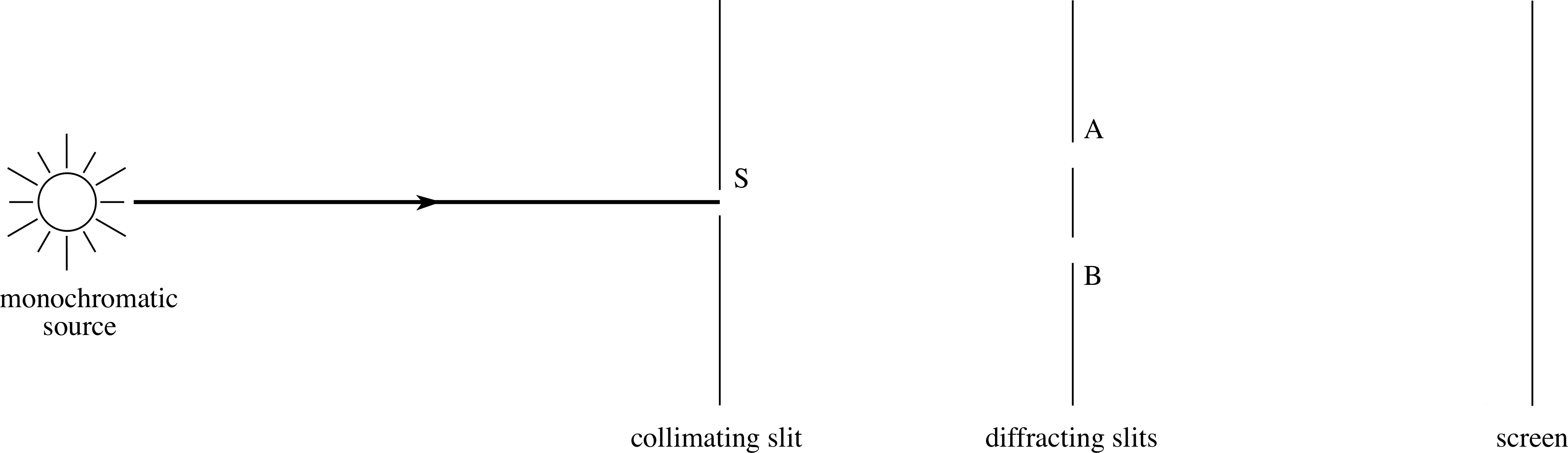
Figure 13 Schematic arrangement in Young’s experiment. Light passing through S will illuminate both A and B, and hence the screen.
In this experiment (shown schematically in Figure 13) light of a single wavelength (monochromatic) from a source passes through a single slit S and falls on a pair of narrow parallel slits A and B, which illuminate a screen. If only one of the slits is open then the screen will be illuminated more or less uniformly. This we can understand easily, whether we regard light as being waves or particles.
If both slits (A and B) are uncovered then we see an interference pattern of parallel bright and dark bands on the screen. i This is just what we expect from a wave. How can we fit photons and energy quanta into this picture? There is no way that particles can produce the dark bands of an interference pattern since at these places particles arrive if either slit is open but not when both slits are open.
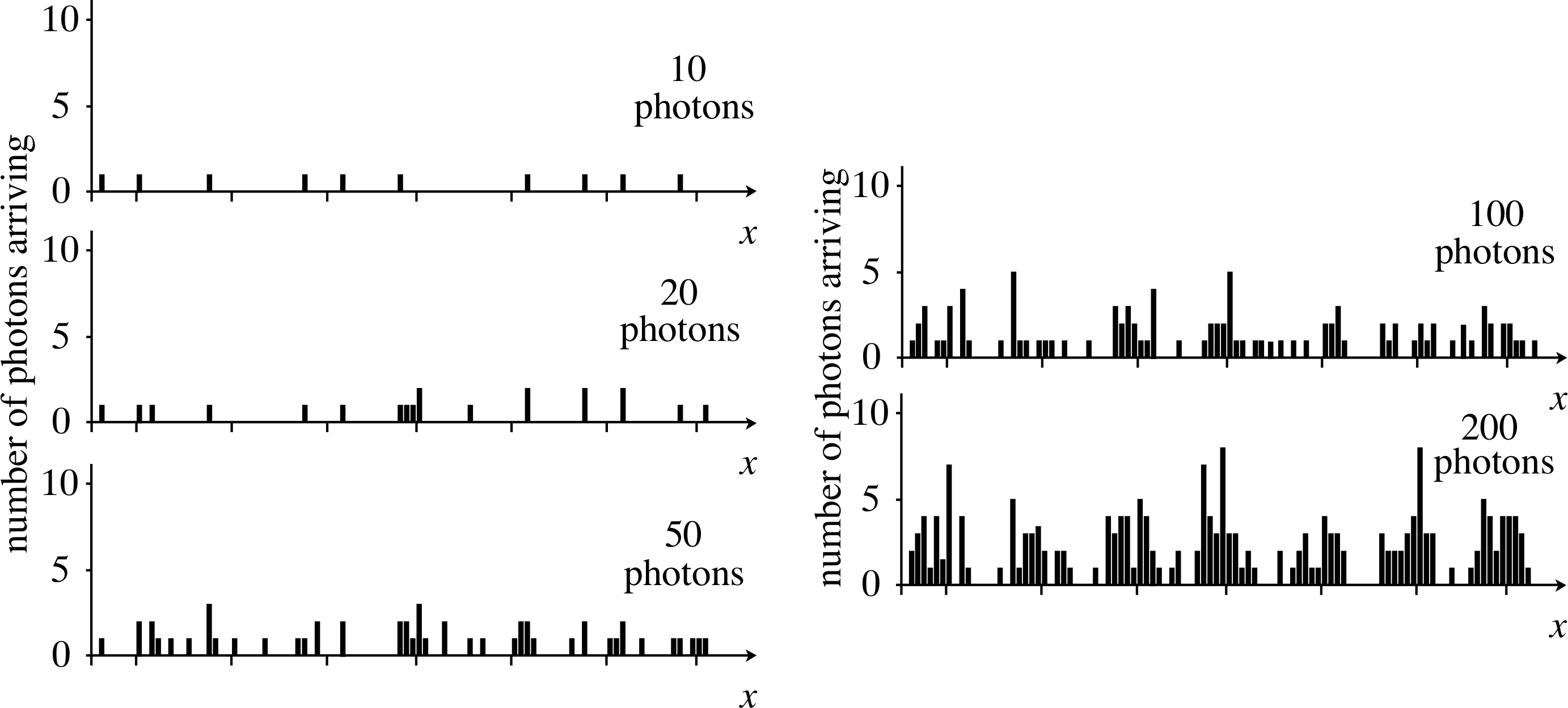
Figure 14a The arrival of photons on the screen in a low intensity version of Young’s experiment. This is a series of histograms, showing how photons may be distributed on the screen as they arrive; situation for 10, 20, 50, 100 and 200 photons.
The way the photons arrive at the screen is shown in Figure 14. When only a few photons have arrived, they appear to be distributed in a random manner, and there is no pattern to be made out. But as more and more arrive, the expected interference pattern gradually becomes more and more apparent.
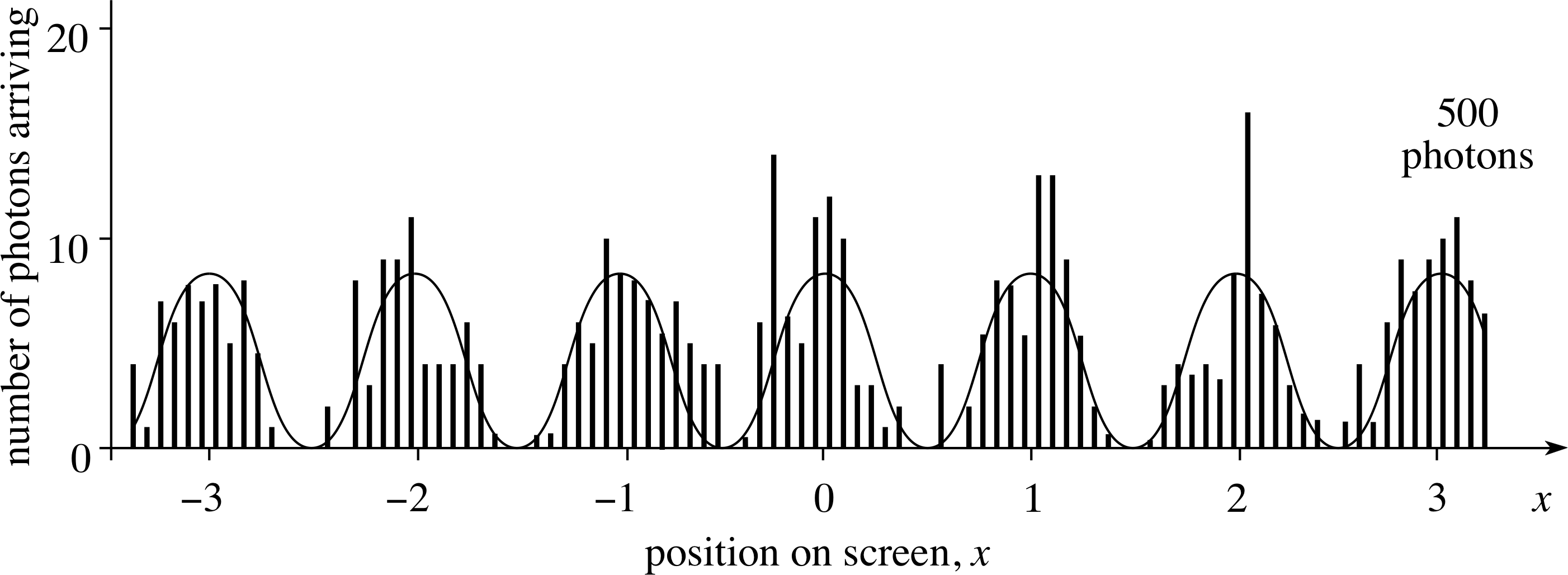
Figure 14b The arrival of photons on the screen in a low intensity version of Young’s experiment. Representation showing how photons may be distributed on the screen as they arrive; situation for 500 photons.
After 500 photons have reached the screen the pattern already bears a strong resemblance to the continuous intensity curve we would expect from the wave model, and which is shown in Figure 14 as a solid line for the 500 photons case. You can see from the Figure 14 that there are several points where photons never arrive – at just those positions where the wave model predicts fully destructive interference.
The overall rate at which the photons arrive at the screen does not affect the shape of the pattern on the screen. Even if the beam is so weak that only one photon is on its way at any one time, the interference pattern is still built up in just the same way – it just takes longer for the pattern to become established. In quantum physics, even when the intensity of a light beam is so weak that its particle–like aspect is apparent, the arrival probability of an individual photon may still be determined by the wave–like aspect of the light. The arrival location of any particular photon cannot be predicted with certainty, only its probability of arrival at any point on the screen.
Quantum physics must therefore deal with probabilities rather than with the certainties inherent in classical physics. The task of setting up an appropriate mathematical basis for quantum physics, so that definite predictions can be made, is a major challenge but this must be left to other FLAP modules.
Question T12
‘Light appears to interact as particles yet travels as waves.’ What experimental evidence supports this statement?
Answer T12
The particle model of interaction is supported by the photoelectric effect, the Compton effect, the black–body spectrum, photon counting experiments and by the absorption and emission of light by atoms.
The wave model is necessary to explain the diffraction and interference of light.
7 Closing items
7.1 Module summary
- 1
-
In the photoelectric effect electrons are ejected from a metal illuminated by light. The electrons have a range of kinetic energies up to a maximum, depending on the metal and on the radiation frequency.
- 2
-
The maximum electron kinetic energy does not depend on the intensity of the light.
- 3
-
The effect can be explained by Einstein’s theory, which assumes that radiation is emitted and absorbed in finite packets, called quanta or photons.
- 4
-
The energy carried by each photon is given by
E = hf(Eqn 2)
where f is the frequency of the radiation and h is a universal constant, called Planck’s constant.
- 5
-
The minimum energy required to remove an electron from the metal is called the work function, usually denoted by ϕ, and is a property of the metal.
- 6
-
Einstein’s photoelectric equationEinstein’s equation for the photoelectric effect expresses the maximum electron energy by
$E = hf − \phi = \dfrac12m_{\rm e}\upsilon_{\rm max}^2$(Eqn 3)
It describes the experimental results exactly.
- 7
-
electromagnetic radiationElectromagnetic radiation, in addition to carrying energy, also carries momentum; the magnitude of the momentum of radiation of energy E is E/c, where c is the speed of light. This relationship is true at the level of a classical wave carrying momentum and also at the photon level.
- 8
-
In the Compton effect, radiation is scattered by matter in such a way that radiation scattered through a particular angle has a particular wavelength, which is longer than the wavelength of the incident radiation. The difference between the incident and scattered radiation is given by
λf − λi = (h/mec)(1 − cos θ)(Eqn 12)
- 9
-
In the Compton effect, the wavelength of the scattered radiation does not depend on the nature of the target.
- 10
-
The relation between scattering angle and the scattered wavelength is accounted for by treating the process in terms of collisions between photons (treated as particles) and electrons in the material.
- 11
-
Both the photoelectric effect and the Compton effect show that in some circumstances light behaves as if it were composed of particles.
- 12
-
Other evidence for the photon model of light comes from the spectrum of Section 5.1black-body radiation, photon counting, short light pulses and from interactions of light with atoms.
- 13
-
The phenomena of Young’s experimentinterference and Young’s experimentdiffraction of light can, however, only be explained by a wave model.
- 14
-
This apparent paradox is partly resolved by assuming that photons in a light beam are distributed according to the intensity of the beam.
- 15
-
The paradox cannot be resolved completely using classical ideas but requires a new theory (quantum physics), which accepts the wave/particle duality displayed by light and matter, and concentrates on predicting the behaviour of physical systems.
7.2 Achievements
Having completed this module, you should be able to:
- A1
-
Define the terms that are emboldened and flagged in the margins of the module.
- A2
-
Describe the essential experimental features of the photoelectric effect.
- A3
-
Explain why the photoelectric effect cannot be explained by classical theory.
- A4
-
Write down the Planck–Einstein formula and explain its significance.
- A5
-
Describe Einstein’s theory of the photoelectric effect, and use it to explain all the experimental features of the effect.
- A6
-
Describe how the momentum carried by light may be observed.
- A7
-
Describe the Compton effect, and its most significant experimental features.
- A8
-
Describe how the wave model of light fails to explain the Compton effect.
- A9
-
Explain the Compton effect in terms of collisions between electrons and photons (without proof of the Compton expression).
- A10
-
Describe the black–body spectrum and explain in general terms (without proof) how its interpretation supports the photon model of light.
- A11
-
Describe the wave/particle duality in the behaviour of light, and explain why such a duality is not necessarily paradoxical.
Study comment You may now wish to take the following Exit test for this module which tests these Achievements. If you prefer to study the module further before taking this test then return to the topModule contents to review some of the topics.
7.3 Exit test
Study comment Having completed this module, you should be able to answer the following questions each of which tests one or more of the Achievements.
Question E1 (A2)
Describe, with a sketch of the apparatus, how you would investigate the photoelectric effect.
Figure 4 Plate D is at a negative potential with respect to plate C, so that electrons from plate C are repelled, and only the more energetic ones are able to reach plate D.
Answer E1
The apparatus is sketched in Figure 4. For a given wavelength light source the voltage of the battery is varied (with plate D at a negative potential with respect to plate C) to find the maximum 2 energy of the ejected electrons.
This is repeated for light sources of different frequencies and a graph of the maximum electron energy against frequency is drawn. Repeating this procedure for different targets should give graphs, all of which have the same slope, allowing Planck’s constant to be found.
(Reread Subsections 2.1 and 2.2 if you had difficulty with this question.)
Question E2 (A3)
Describe those features of the photoelectric effect that cannot be explained by the wave model of light.
Answer E2
The maximum electron energy is independent of the light intensity and dependent only on the light frequency, and there is a critical frequency below which photoelectrons are not emitted. Also there is no time delay in emission, irrespective of intensity.
(Reread Subsections 2.1 and 2.2 if you had difficulty with this question.)
Question E3 (A4)
The yellow light emitted from sodium has a wavelength of 589 nm. Calculate the energy of its photon, in joules and electronvolts.
Answer E3
589 nm = 589 × 10−9 m. The corresponding frequency is c/λ = 3 × 10⁸ m s−1/589 × 10−9 m = 5.09 × 10¹⁴ Hz and the energy is
hf = 6.63 × 10⁻³⁴ J s × 5.09 × 10¹⁴ Hz = 3.37 × 10⁻¹⁹ J = 2.11 eV.
(Reread Subsection 2.2 if you had difficulty with this question)
Question E4 (A5)
The work function of sodium is 2.0 eV. Find (a) its threshold wavelength, (b) the maximum energy of ejected electrons when it is illuminated by light of wavelength 4.5 × 10⁻⁷ m, (c) the stopping voltage for this wavelength.
Answer E4
(a) The threshold energy, i.e. the minimum energy required to eject electrons from the metal, is the work function ϕ, which is 2.0 eV = 3.2 × 10⁻¹⁹ J. The frequency of radiation of this photon energy is found by dividing the energy by h, giving ϕ/h, and the wavelength by dividing this into c, giving hc/ϕ, which is 6.2 × 10⁻⁷ m.
(b) The maximum energy of ejected electrons when the surface is illuminated by light of wavelength 4.5 × 10⁻⁷ m is obtained by subtracting the work function from the incident photon energy, as in Einstein’s photoelectric equation:
$hf - \phi = \frac12m_{\rm e}\upsilon_{\rm max}^2$(Eqn 3)
i.e.$E_{\rm max} = \dfrac12m_{\rm e}\upsilon_{\rm max}^2 = hf - \phi = \dfrac{hc}{\lambda} - \phi$
In this case we have:
$E_{\rm max} = \rm \dfrac{6.63\times10^{-34}\,J\,s\times3.00\times10^8\,m\,s^{-1}}{4.5\times10^{-7}\,m} -3.2\times10^{-19}\,J = 1.2\times10^{-19}\,J = 0.76\,eV$
(c) The stopping voltage is given by:
$\frac12m_{\rm e}\upsilon^2 = eV_{\rm s}$(Eqn 1)
so$V_{\rm s} = \dfrac{E_{\rm max}}{e} = \rm 0.76\,V$
(Reread Subsections 2.1 and 2.2 if you had difficulty with this question.)
Question E5 (A6)
(a) The rate at which solar energy arrives at the Earth’s surface per unit area is 1.4 kW m−2. What is the radiation pressure due to this? (b) If you assume that the average photon energy corresponds to a wavelength of 600 nm, how many arrive per second on a square metre?
Answer E5
(a) The momentum transferred per unit area per unit time, and so the pressure, is obtained by dividing the energy transfer rate by c. So if all the light is absorbed, the pressure is 1.4 × 10³ J s−1 m−2/3 × 108 m s−1 = 4.7 × 10⁻⁶ N m−2.
(b) The energy of a photon of wavelength 600 nm is
hc/λ = 6.63 × 10⁻³⁴ J s × 3.00 × 10⁸ m s−1/600 × 10−9 m = 3.32 × 10⁻¹⁹ J
and the arrival rate is
1.4 × 10³ J m−2 s−1/3.31 × 10−19 J = 4.2 × 10²¹ m−2 s−1
(Reread Section 3 if you had difficulty with this question.)
Question E6 (A7, A8 and A9)
Which features of the Compton effect cannot be explained by the wave model of light, but can be explained by the photon model?
Answer E6
The features are the five characteristics listed below, and which are discussed in Subections 4.2 and 4.3.
- 1
-
The scattered radiation consists of two wavelengths, the original one λi and an additional one λf.
- 2
-
λf is always greater than or equal to λi.
- 3
-
λf depends on the scattering angle.
- 4
-
λf does not depend on the material of the target.
- 5
-
λf obeys the angular dependence predicted by Equation 12,
λf − λi = (h/mec)(1 − cos θ)(Eqn 12)
Question E7 (A7 and A9)
A gamma–ray photon from the radioactive isotope 13766Cs has an energy of 2 keV. If it is scattered by a free electron through an angle of 30°, what will be its final energy?
Answer E7
See Subsection 4.2.
An energy of 662 × 103 eV = 1.06 × 10⁻¹³ J corresponds to a wavelength of hc/E = 1.873 × 10⁻¹² m.
Using Equation 12,
λf − λi = (h/mec)(1 − cos θ)(Eqn 12)
λf − λi = 2.43 × 10−12 m × (1 − 0.866) = 3.25 × 10⁻¹³ m
soλf = (1.873 + 0.325) × 10−12 m = 2.20 × 10⁻¹² m.
To find the energy we reverse the calculation at the beginning of this question:
E = hc/λf = 0.904 × 10⁻¹³ J = 564 × 103 eV = 564 keV
Question E8 (A10)
What is meant by the term black-body radiation? Explain in general terms (without proof) how its interpretation supports the photon model of light.
Figure 12 The continuous emission spectrum from an idealized hot body, the so–called black–body radiation. The vertical scale shows the spectral brightness of the surface and the horizontal scale shows the wavelength. The spectrum from the same body at two different temperatures (T2 > T1) is shown. Note that the peak of the spectrum shifts to shorter wavelengths as the temperature is increased.
Answer E8
The radiation coming from an idealized hot body is called a black–body spectrum. For classical electromagnetic waves within an enclosure, the energy density rises without limit as the frequency increases. To deal with this, Planck assumed that the wall contained oscillators with discrete energy states, and that interactions between these oscillators and the radiation were quantized. This model correctly predicted the shape of the black–body spectrum.
(Reread Subsection 5.1 if you had difficulty with this question.)
Question E9 (A11)
Light can be regarded as being composed either of waves or particles. Under what circumstances would you use each model?
Answer E9
The propagation of light requires the wave model but its interactions with matter require the particle model. Light shows the features of both models and a full understanding requires the use of quantum physics.
(Reread Section 6 if you had difficulty with this question.)
Study comment This is the final Exit test question. When you have completed the Exit test go back and try the Subsection 1.2Fast track questions if you have not already done so.
If you have completed both the Fast track questions and the Exit test, then you have finished the module and may leave it here.
7.4 Further reading
The following two books are both general reading, but are worthwhile for any physicist at any stage of life.
‘Subtle is the Lord...’: The Science and Life of Albert Einstein, by Abraham Pais, Oxford University Press, 1982. This is an excellent account of Einstein’s life, with the emphasis on the science, and has a good history of the development of the photon concept.
‘QED The Strange Theory of Light and Matter’, by R. P. Feynman, Penguin Books, 1990. Richard Feynman was one of the most original scientists of the century, and one of the inventors of the theory described here. It goes further than this module, but contains hardly any mathematics, having been written for the intelligent lay person.
Study comment Having seen the Fast track questions you may feel that it would be wiser to follow the normal route through the module and to proceed directly to the following Ready to study? Subsection.
Alternatively, you may still be sufficiently comfortable with the material covered by the module to proceed directly to the Section 7Closing items.