MATH 6.3: Solving second order differential equations |
PPLATO @ | |||||
PPLATO / FLAP (Flexible Learning Approach To Physics) |
||||||
|
1 Opening items
1.1 Module introduction
Suppose that we are interested in the behaviour of a mass m, free to bob up and down along the y–axis on the end of a spring of force constant k, and also subject to a damping (or resistive) force the magnitude of which is proportional to the speed of the mass, as well as to an externally imposed periodic force in the y–direction given by Fy = F0 sin(Ωt) where F0 is a positive constant. (Fy is commonly abbreviated to F to avoid unnecessary confusion with the subscripts.) The equation of motion of the mass is obtained by applying Newton’s second law. If y is the displacement of the mass from equilibrium, then we have
$m\dfrac{d^2y}{dt^2} = -ky - b\dfrac{dy}{dt} + F_0\sin ({\it\Omega}t)$(1)
All the forces acting on the mass have been added together on the right–hand side of Equation 1, and are as follows:
$\begin{align}& -ky && \text{(the restoring force exerted by the spring);}\\& -b\dfrac{dy}{dt}, \text{where } b \text{ is a positive constant} && \text{(the damping force);}\\& F_0\sin({\it\Omega}t) && \text{(the periodic applied force).}\end{align}$
Equation 1 is an example of a second-order linear differential equation. It belongs to a category of linear differential equations known as linear equations with constant coefficients, where the dependent variable and its derivatives are multiplied by constants (not by functions of the independent variable).
The most general second–order equation of this sort can be written as
$a\dfrac{d^2y}{dt^2} + b\dfrac{dy}{dx} + cy = f(t)$(2)
where a, b, c are constants and a ≠ 0; it is equations of this type that will be discussed in this module.
The simplest of this type of equation is one for which b and c are zero, so that the equation becomes
$a\dfrac{d^2y}{dt^2} = f(t)$(3)
This can be solved by direct integration, as will be explained in Subsection 2.1. Another relatively simple case arises when we have zero on the right–hand side of Equation 2, instead of a function of t, so that
$a\dfrac{d^2y}{dt^2} + b\dfrac{dy}{dx} + cy = 0$, where a, b, c are constants and a ≠ 0(4)
Equations of this type (known as linear homogenous equations) have innumerable applications in physics; they arise, for example, in the discussion of simple harmonic motion and the analysis of a.c. circuits. i Much of this module (Subsection 2.2Subsections 2.2 to Subsection 2.52.5) is therefore devoted to finding solutions to various forms of Equation 4.
Subsection 2.6 shows you how to solve some equations of the type given in Equation 2 for some different forms of f (t). The method explained there will then be used in Subsection 2.7 to find the general solution of equations of the type
$m\dfrac{d^2y}{dt^2} = -ky - b\dfrac{dy}{dt} + F_0\sin({\it\Omega}t)$(Eqn 1)
Study comment Having read the introduction you may feel that you are already familiar with the material covered by this module and that you do not need to study it. If so, try the following Fast track questions. If not, proceed directly to the Subsection 1.3Ready to study? Subsection.
1.2 Fast track questions
Study comment Can you answer the following Fast track questions? If you answer the questions successfully you need only glance through the module before looking at the Subsection 3.1Module summary and the Subsection 3.2Achievements. If you are sure that you can meet each of these achievements, try the Subsection 3.3Exit test. If you have difficulty with only one or two of the questions you should follow the guidance given in the answers and read the relevant parts of the module. However, if you have difficulty with more than two of the Exit questions you are strongly advised to study the whole module.
Question F1
The angular displacement θ of the bob of a simple pendulum satisfies the equation of motion
$a\dfrac{d^2\theta}{dt^2} + b\dfrac{d\theta}{dt} + c\theta = 0$
(a) Find the general solution of this equation if a = 0.1 kg, b = 0.2 kg s−1 and c = 1.0 kg s−2.
(b) Find the particular solution if the bob is hit when in its rest position θ = 0 such that it is given an angular speed $\dfrac{d\theta}{dt} = 0.3\,{\rm rad\,s^{-1}}$ at t = 0.
(c) Sketch this solution as a function of t.
Answer F1
(a) The discriminant (b2 − 4ac) of this equation is equal to [(0.2)2 − 4 × 0.1 × 1] kg2 s−1 = −0.36 kg2 s−2 < 0. Thus the general solution is (from Equation 37 and 38)
y (t) = exp(−γt/2)[(B cos(ωt) + C sin(ωt)](37)
withγ = b/a(38a)
and$\omega = \sqrt{4ac-b^2}{\large/}(2a)$(38b)
where γ = −b/(2a) = −0.2 kg2 s−1/(2 × 0.1 kg) = −1.0 s−2
and$\omega = \sqrt{4ac-b^2}{\large/}(2a) = \left[(1/0.2)\sqrt{0.4-0.04\os}\right]\,{\rm s^{-1}} = 3\,{\rm s^{-1}}$
If these values are substituted into the original equation we find:
θ = exp[−(1.0 s−1)t] {B cos[(3 s−1)t] + C sin[(3 s−1)t]}
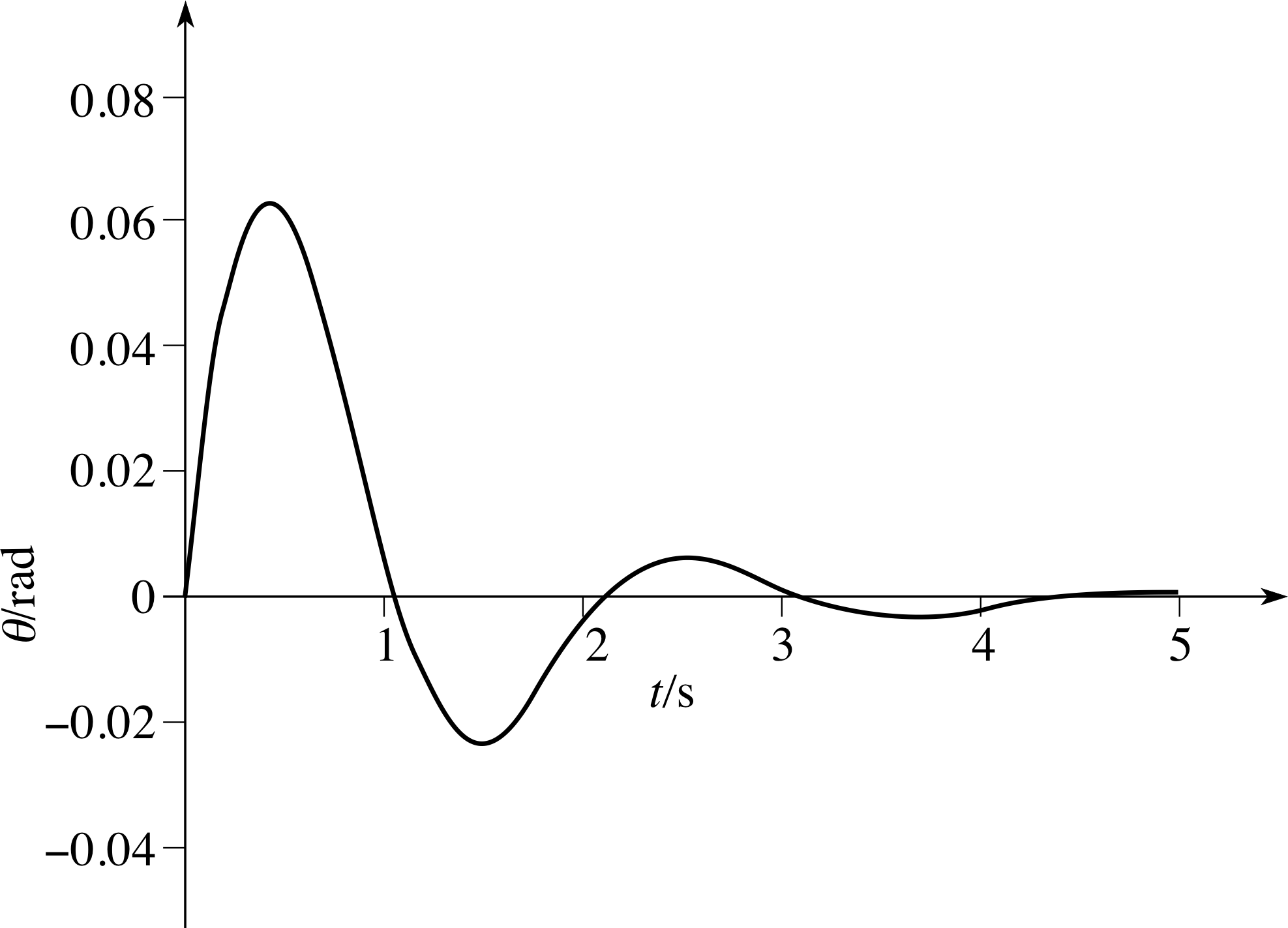
Figure 9 See Answer F1.
(b) If we substitute the condition θ = 0 at t = 0, we find B = 0. So the solution is of the form
θ = Cexp(γt) sin(ωt). If this is differentiated using the product rule, we find
$\dfrac{d\theta}{dt} = \gamma C\exp(\gamma t)\sin(\omega t) + \omega C\exp(\gamma t)\cos(\omega t)$
and if we substitute dθ/dt = 0.3 rad s−1 at t = 0, we find C = 0.1 rad, so the particular solution is
θ = (0.1 rad) exp[−(1.0 s−1)t] sin[(3 s−1)t].
(c) The sketch is shown in Figure 9.
Question F2
Find the general solution to the equation
$\dfrac{d^2x}{dt^2} + 5\dfrac{dx}{dt} + 6x = 2t^2$ i
Answer F2
We first find the complementary function, i.e. the general solution to
$\dfrac{d^2x}{dt^2} + 5\dfrac{dx}{dt} + 6x = 0$
The discriminant of the auxillary equation is
b2 − 4ac = 25 − 24 = 1 > 0
Thus the general solution is (from Equation 33),
y (t) = B exp(p1t) + C exp(p2t)(Eqn 33)
x = B exp(p1t) + C exp(p2t)
where p1 and p2 are the roots of the auxiliary equation p2 + 5p + 6 = 0. These roots are p1 = −2, p2 = −3. So the complimentary function is
Be−2t + Ce−3t
To find a particular solution, we try a solution of the form Ht2 + Kt + L, where H, K, L are constants to be determined. On substitution, we find
2H + 5 (2Ht + K) + 6 (Ht2 + Kt + L) = 2t2
which is an identity provided that 6H = 2, 10H + 6K = 0 and 2H + 5K + 6L = 0, i.e. H = 1/3, K = −5/9, L = 19/54.
So$\dfrac{t^2}{3}-\dfrac{5t}{9}+\dfrac{19}{54}$
is a particular solution. The general solution is given by the sum of the particular solution and the complementary function, and hence is
$x = B{\rm e}^{-2t} + C{\rm e}^{-3t} + \dfrac{t^2}{3}-\dfrac{5t}{9}+\dfrac{19}{54}$
1.3 Ready to study?
Study comment In order to study this module you will need to be familiar with the following terms: degree_of_a_polynomialdegree (of a polynomial), exponential function, general solution, initial condition, linear differential equation and particular solution. You will also need to be familiar with various trigonometric identities (although we will repeat them here); to be able to solve first–order differential equations by direct integration (which requires a fair knowledge of integration methods); to know how to check a proposed solution_mathematicalsolution to a differential equation by substitution (which requires good differentiation skills); and to be able to use initial conditions to obtain a particular solution from a general solution. To appreciate the physical significance of some of the equations appearing in this module, you should know how to use Newton’s second law to write down a differential equation describing the motion of an object if you are given information about the forces acting on it. Some familiarity with simple harmonic motion (SHM) would be particularly useful. If you are uncertain about any of these terms, you can review them now by reference to the Glossary, which will also indicate where in FLAP they are developed. The following questions will allow you to establish whether you need to review some of these topics before embarking on this module.
Question R1
Find the general solution to the differential equation
$\dfrac{dy}{dx} = \dfrac{x}{1+x^2}$
Answer R1
This differential equation may be solved by direct integration. The solution is
$\displaystyle y = \int\dfrac{x\,dx}{1+x^2}$
To evaluate the integral, make the substitution u = 1 + x2. This gives
$\displaystyle y = \dfrac12 \int\dfrac{du}{u} = \dfrac12\loge u + C = \dfrac12\loge(1+x) + C$
where C is an arbitrary constant
(If you did not know how to solve this differential equation, consult direct integration in the Glossary.)
Question R2
If y = 4 ex/2 cos 2x, calculate dy/dx and d2y/dx2.
Answer R2
We use the product_rule_of_differentiationproduct rule to differentiate y. This gives us
$\dfrac{dy}{dx} = 4\times \frac12 {\rm e}^{x/2}\cos(2x) + 4\times {\rm e}^{x/2}\times[-2\sin(2x)] = {\rm e}^{x/2}[2\cos(2x)-8\sin(2x)]$
Differentiating dy/dx (again using the product rule) gives us
$\dfrac{d^2y}{dx^2} =\frac12 {\rm e}^{x/2}[2\cos(2x)-8\sin(2x)] + {\rm e}^{x/2}[-4\sin(2x)-16\cos(2x)] = {\rm e}^{x/2}[-15\cos(2x)-8\sin(2x)]$
(If you could not do this question, you should consult differentiation in the Glossary.)
Question R3
Show by substitution that $y = \frac14(2x-3) + A{\rm e}^{-x}$, where A is an arbitrary constant, is a solution to
$\dfrac{d^2y}{dx^2} + 3\dfrac{dy}{dx} + 2y = x$
Is it a general solution?
Answer R3
If $y = \frac14(2x-3) + A{\rm e}^{-x}$, then $\dfrac{dy}{dx} = \dfrac12 - A{\rm e}^{-x}$ and $\dfrac{d^2y}{dx^2} = A{\rm e}^{-x}$.
Substituting these expressions into the left–hand side of the differential equation gives us
$A{\rm e}^{-x} + \frac32 - 3A{\rm e}^{-x} + \frac12(2x-3) + 2A{\rm e}^{-x}$
which is identically equal to x, the right–hand side. So this expression is a solution. It cannot be the general solution, however, as it contains only one arbitrary constant, A, and the general solution to a second–order differential equation must contain two arbitrary constants.
(If you could not do this question, you should consult solution_mathematicalsolution (of a differential equation) in the Glossary.)
Question R4
In answering this question, you should make use only of trigonometric identities, you should not use your calculator. i
(a) If cos θ = 1/3, what is the value of sin θ, given 0 < θ < π/2 ?
(b) If cos θ = 1/3 and sin ϕ = −1/2, what is the value of cos(θ + ϕ), given 0 < θ < π/2, π < ϕ < 3π/2?
Answer R4
(a) If cos θ = 1/3, then we may use the identity
cos2 θ + sin2 θ = 1
to deduce that $\sin\theta = \sqrt{1-(1/9)\os} = \pm(2\sqrt{2\os})/3$
Since 0 < θ < π/2, sin θ must be positive; so
$\sin\theta = (2\sqrt{2\os})/3$
(b) To evaluate cos(θ + ϕ), we may use the identity
cos(θ + ϕ) = cos θ cosϕ − sin θ sin ϕ
We are given the values of cos θ and sin ϕ, and from part (a), we know that $\sin\theta = \frac23\sqrt{2\os}$. Therefore we need to find cos ϕ. Using the identity cos2 ϕ + sin2 ϕ = 1, we deduce that
$\cos\varphi = \sqrt{1-\frac14\os} = \pm\frac12\sqrt{3\os}$
Since π < ϕ < 3π/2, cos ϕ must be negative; so $\cos\varphi = \frac12\sqrt{3\os}$.
Substituting all these values into the identity above, we find
$\cos(\theta+\varphi) = \left.\left(2\sqrt{2\os}-\sqrt{3\os}\right)\middle/6\right.$
(If you are unfamiliar with these trigonometric identities, or with the signs of sine and cosine functions for different ranges of their arguments, you should consult trigonometric functions in the Glossary.)
Question R5
In each of the two following expressions for y, use the given initial conditions to calculate values for the arbitrary constants A and B.
(a) y = (At + B)e−2t; where y = 1 and dy/dt = 3 at t = 0.
(b) y = A cos 2x + B sin 2x; where y = 4 and dy/dx = −2 at x = 0.
Answer R5
(a) If y = (At + B)e−2t, then dy/dt = (−2At − 2B + A)e−2t. Substituting the values given into these equations, and putting t = 0, we find 1 = B and 3 = −2B + A (note that e0 = 1). So B = 1 and A = 5.
(b) If y = A cos(2x) + B sin(2x), then dy/dx = −2A sin(2x) + 2B cos(2x). Substituting the values given into these equations, and putting x = 0, we find 4 = A and −2 = 2B (note that sin 0 = 0, cos 0 = 1). So A = 4 and B = −1.
Question R6
An object of mass m is free to move along a line; its displacement from the origin is denoted by x. It is acted on by three forces: a restoring force, the magnitude of which is proportional to the magnitude of x; a resistive (or damping) force, the magnitude of which is proportional to the cube of the object’s speed; and a constant force of magnitude F0 acting in the negative x–direction. Use Newton’s second law to write down the second–order differential equation that x must satisfy.
Answer R6
The equation of motion of the object is obtained from Newton’s second law by using
$m\dfrac{d^2x}{dt^2} = F_x$
where Fx on the right–hand side is the sum of the components_of_a_vectorcomponents of the forces acting in the x–direction. A restoring force is one which is in the opposite direction to x; since the magnitude of this force is proportional to the magnitude of x, we may write the force as −kx, where k is a positive constant (so that it is negative when x is positive and vice versa). A resistive (or damping) force is always in the opposite direction to the velocity (dx/dt) of the object; in this case this force must take the form −c (dx/dt)2, where c is a positive constant. The constant force must be written as minus Fx, since it acts in the negative x–direction. So the equation of motion is
$\dfrac{d^2x}{dt^2} = -kx - c\left(\dfrac{dx}{dt}\right) - F_0$
(If you could not do this question, you can still study this module, but the physical significance of some of the differential equations discussed here may not be clear to you.)
2 Methods of solution for various second–order differential equations
Notation Very often in the problems that arise in physics the independent variable is time, and so, when discussing a general type of differential equation, the independent variable is denoted by t and the dependent variable by y. However, in some of the examples, drawn from specific problems in physics, we will use the notation for the variables that is appropriate to the situation. Bear in mind that the quantity being differentiated will always be the dependent variable.
2.1 Classifying second–order differential equations
There is such a wide variety of second–order differential equations that it is useful to divide them into various categories, and in this subsection we will introduce some terminology that arises when we do so. You are probably already familiar with the distinction between linear and non-linear differential equations. The most general linear second–order differential equation is of the form
$a(t)\dfrac{d^2y}{dt^2} + b(t)\dfrac{dy}{dx} + c(t)y = f(t)$
where a (t), b (t), c (t) and f (t) are functions of t.
However, in many of the second–order linear equations that you will encounter in your study of physics the dependent variable and its derivatives appear multiplied only by constants rather than functions of t. Such an equation is known as a linear differential equation with constant coefficients and has the form
$a\dfrac{d^2y}{dt^2} + b\dfrac{dy}{dx} + cy = f(t)$(5) i
Equation 5 is easiest to solve when its right–hand side is zero, i.e. when
$a\dfrac{d^2y}{dt^2} + b\dfrac{dy}{dt} + cy = 0$(6)
As you see, all the terms in Equation 6 contain the dependent variable y or a derivative of y; for that reason, an equation of this form is called a linear homogeneous differential equation. We will discuss equations of this sort in Subsection 2.3Subsections 2.3, Subsection 2.42.4 and Subsection 2.52.5. If f (t) in Equation 5 is not zero, then the equation is called a linear inhomogeneous differential equation (as there is now a term in the equation which does not involve the dependent variable y). Equation 6 is relatively easy to solve, whereas the ease with which we are able to solve Equation 5 is crucially dependent on the form of the function f (t).
Question T1
State whether the following differential equations are linear with constant coefficients and, if so, whether they are homogeneous or inhomogeneous:
(a) $\dfrac{d^2y}{dx^2} = x-3y$, (b) $x\dfrac{d^2y}{dx^2} + 2\dfrac{dy}{dx}+ y = 0$, (c) $\dfrac{d^2x}{dt^2} - 5\dfrac{dx}{dt} = 6x$
Answer T1
(a) This is linear with constant coefficients; it is inhomogeneous (because of the term in x).
(b) The coefficient of d2y/dx2 is not a constant, so the equation does not have constant coefficients.
(c) This is a linear with constant coefficients, and homogeneous.
We will first dispose of the easiest of all second–order differential equations – those that may be solved by direct integration. This is the subject of the next subsection.
2.2 Equations of the form d2y/dt2 = f (t); direct integration
You should already know how to solve a first–order differential equation i of the form
$\dfrac{dy}{dt} = f(t)$(7)
where the derivative of the dependent variable is equal to a function of the independent variable. This equation may be integrated directly, to give
$y = \Int f(t)\,dt$(8)
The indefinite integral will involve one arbitrary constant of integration, this indicates that Equation 8 gives us the general solution to Equation 7.
It is just as straightforward to solve a second–order differential equation of the form
$\dfrac{d^2y}{dt^2} = f(t)$(9)
where the second derivative of the dependent variable is equal to a function of the independent variable. Here, we simply integrate directly twice. Recalling that d2y/dt2 is the derivative of dy/dt, we see that if we integrate both sides of Equation 9, we obtain
$\dfrac{dy}{dt} = \Int f(t)\,dt = F(t) + A$(10)
where F (t) is an indefinite integral i of f (t) (i.e. F (t) is a function such that F ′ (t) = dF (t)/dt = f (t)), and A is a constant of integration. If we integrate Equation 10 again we obtain:
$y = \Int(F(t) + A)\,dt = G(t) + At + B$(11)
where G (t) is an indefinite integral of F (t), and B is another constant of integration. We see that Equation 11 contains two arbitrary constants, A and B; this indicates that it is the general solution to Equation 9.
Equations which can be directly integrated often arise when considering objects that are moving along a line. For instance, an object moving along the x–axis, with position coordinate x and acceleration ax(t), a known function of time, satisfies the equation
$\dfrac{d^2x}{dt^2} = a_x(t)$(12) i
The following example illustrates this.
Example 1
A car is travelling in the x–direction along a straight road. At time t = 0, it starts to accelerate, and for the next 8 s, its acceleration ax(t) is given by ax(t) = a + bt. If a = 2.00 m s−2, b = 0.50 m s−3 and the car’s velocity is 5.00 m s−1 at t = 0, how far does the car travel during the 8 s period?
Solution
We must first solve the differential equation
$\dfrac{d^2x}{dt^2} = a + bt$ i
where x = x (t) is the position of the car and we take the origin to be the position of the car at t = 0, so that x = 0 at t = 0. Integrating once gives us
$\dfrac{dx}{dt} = \Int(a+bt)\,dt = at + b\left(\dfrac{t^2}{2}\right) + A = at + \dfrac b2 t^2 + A$
where A is an arbitrary constant. On substituting dx/dt = 5.00 m s−1 at t = 0 into this equation, we find A = 5 m s−1.
Integrating dx/dt to find x gives us
$\displaystyle x = \int\left(at + \dfrac b2 t^2 + A\right) = \dfrac{at^2}{2} + \dfrac{bt^3}{6} + At + B$
where B is an arbitrary constant. If we substitute x = 0 at t = 0, we find B = 0.
So$x = (0.5\,{\rm m\,s^{-3}})\dfrac{t^3}{6} + (2.0\,{\rm m\,s^{-2}})\dfrac{t^2}{2} + (5.0\,{\rm m\,s^{-1}})t$
Therefore at t = 8 s, we find that the car has travelled 146.6 m.
Sometimes, instead of being given information directly about the acceleration of the object, you may be given the force Fx(t) acting on it as a function of time. However, since Fx(t) = max(t), where m is the mass of the object, it is very easy to write down a differential equation of the form given in Equation 12.
$\dfrac{d^2x}{dt^2} = a_x(t)$(Eqn 12)
Such a differential equation, arising from an application of Newton’s second law, is often called an equation of motion.
Try the following question, which illustrates another example.
Question T2
An object of mass 2 kg, which is constrained to move along the x–axis, is subject to a force Fx(t) = F0cos(Ωt), i acting along the x–axis (in the direction of increasing x), where F0 = 4 N and Ω = 2 s−1. At time t = 0, the object’s displacement is +3 m and its velocity is +1 m s−1. Find its displacement as a function of time.
Answer T2
If the displacement of the object is x, the equation of motion is
$m\dfrac{d^2x}{dt^2} = F_0\cos({\it\Omega}t)$, i.e. $\dfrac{d^2x}{dt^2} = \dfrac{F_0}{m}\cos({\it\Omega}t)$
Integrating once gives us
$\displaystyle \dfrac{dx}{dt} = \int\dfrac{F_0}{m}\cos{\it\Omega}t)\,dt = \int\dfrac{F_0}{m{\it\Omega}}\sin({\it\Omega}t) + A$
and integrating a second time we find
$\displaystyle x = \int\left[\dfrac{F_0}{m{\it\Omega}}\sin({\it\Omega}t) + A\right]\,dt = \dfrac{F_0}{m{\it\Omega}^2}\sin({\it\Omega}t) + At + B$
where A and B are arbitrary constants. At t = 0, dx/dt = 1 m s−1; so A = 1 m s−2. At t = 0, x = 3 m;
so$3\,{\rm m} = -\dfrac{F_0}{m{\it\Omega}^2} + B$, so B = (7/2) m. Thus the particular solution giving the object’s displacement is
$x = \left(\dfrac{-1\,{\rm m}}{2}\right)\cos[(2\,{\rm s^{-1}})t] + (1\,{\rm m\,s^{-1}})t + 7\,{\rm m}$
2.3 The equation for simple harmonic motion: d2y/dt2 + ω2y = 0
We will now make a start at finding solutions of Equation 6, i
$a\dfrac{d^2y}{dt^2} + b\dfrac{dy}{dt} + cy = 0$(Eqn 6)
In this subsection (and the next), we will look at the simplified case where b = 0, so that Equation 6 takes the form
$a\dfrac{d^2y}{dt^2} + cy = 0$(13)
In Equation 13, a ≠ 0 (so the equation is of second order) and c ≠ 0. (If c were zero, we could solve the equation by direct integration.) Since a ≠ 0, we can divide both sides of the equation by a, and write h = c/a to give:
$\dfrac{d^2y}{dt^2} + hy = 0$(14)
You will see shortly that the form of solution of Equation 14 depends on whether the constant h is positive or negative. We will consider these two possibilities separately, starting with the case of positive h. (The case of negative h will be discussed in Subsection 2.4.) If h is positive, we can make it clear that this is so by writing h = ω02, so that Equation 14 becomes:
$\dfrac{d^2y}{dt^2} + \omega_0^2y = 0$ (SHM equation)(15) i
Before discussing the solutions to Equation 15, we will emphasize the importance of this equation in physics. It is the equation of motion of any object undergoing simple harmonic motion (SHM) – motion where the force acting on the object is proportional to the object’s displacement from some point and acts in the opposite direction to the displacement. For this reason, Equation 15 is often known as the SHM equation.
You may already know that an object undergoing SHM executes oscillations and we will see shortly that the period of the oscillations depends on the parameter ω0 which is known as the angular frequency in the context of Equation 15.
So it is important that whenever you encounter a case of SHM, you should be able to rewrite the differential equation describing the physical situation in the form of Equation 15, and so find an expression for ω0 in terms of the parameters appearing in the problem. The following question gives you practice in this.
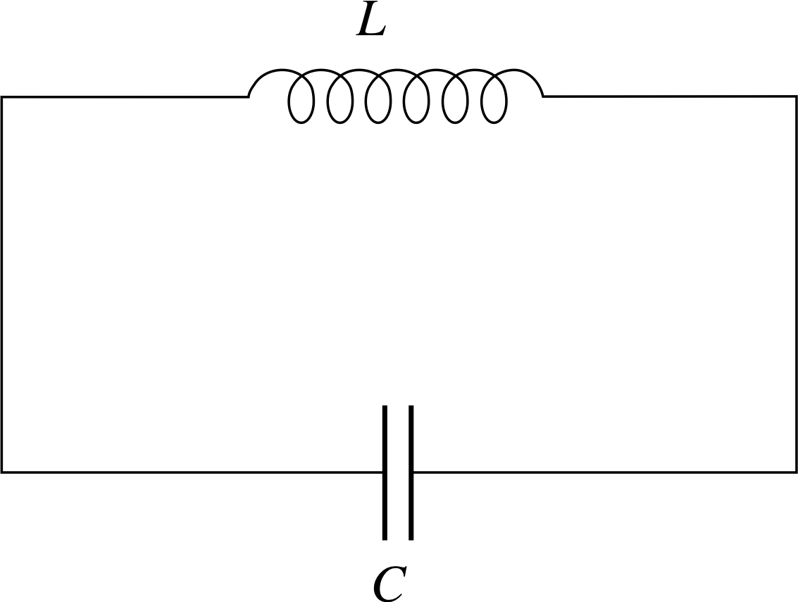
Figure 1 See Question T3(a).
Question T3
Rewrite each of the following equations in the form of Equation 15,
$\dfrac{d^2y}{dt^2} + \omega_0^2y = 0$(Eqn 15)
and so find an expression for ω0:
(a) $L\dfrac{d^2I}{dt^2} + I = 0$
This equation describes the way in which the current I varies with time in a circuit containing an inductor L and a charged capacitor C, as shown in Figure 1.
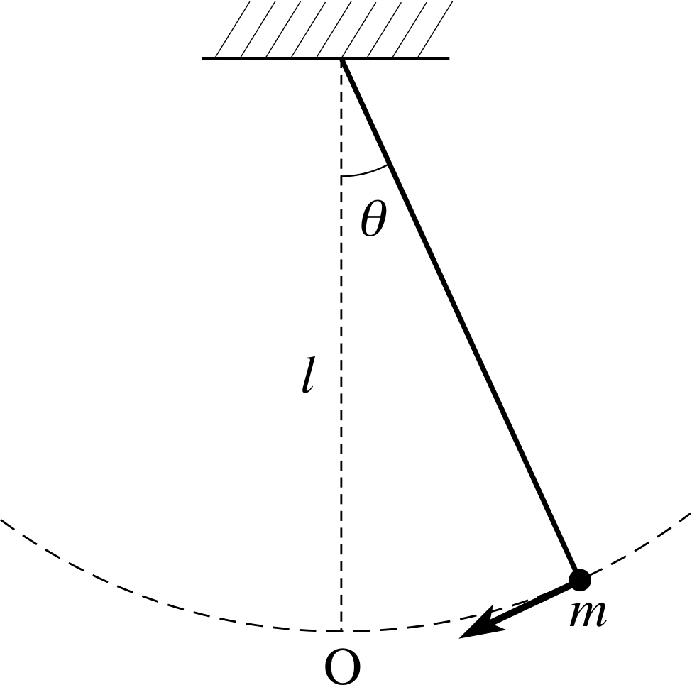
Figure 2 See Question T3(b).
(b) $ml\dfrac{d^2\theta}{dt^2} = -mg\theta$
This equation describes the motion of a simple pendulum – a mass m suspended from a fixed point by a string of length l, as shown in Figure 2.
Answer T3
(a) Rewriting this equation in the form of Equation 15,
$\dfrac{d^2y}{dt^2} + \omega_0^2 y = 0$(Eqn 15)
it becomes
$\dfrac{d^2I}{dt^2} + \dfrac{1}{LC}I = 0$
So$\omega_0 = 1/\sqrt{LC\os}$
(b) Rewriting this equation in the form of Equation 15, it becomes
$\dfrac{d^2\theta}{dt^2} + \dfrac gl \theta = 0$
So$\omega_0 = 1/\sqrt{g/l\os}$
It is not too difficult to guess the general solution of Equation 15,
$\dfrac{d^2y}{dt^2} + \omega_0^2y = 0$(Eqn 15)
Any solution of this equation must be a function such that when we differentiate it twice, we recover the function itself, multiplied by −ω02. This should remind you of a cosine or a sine function. In fact, both cos(ω0t) and sin(ω0t) have precisely this property, as does any function of the form Bcos(ω0t) + C sin(ω0t), where B and C are arbitrary constants.
✦ Show that y = B cos(ω0t) + C sin(ω0t) is a solution to Equation 15.
✧ If we differentiate y once we obtain
$\dfrac{dy}{dt} = -\omega_0B\sin(\omega_0t) + \omega_0C\cos(\omega_0t)$
Differentiate again and we obtain
$\dfrac{d^2y}{dt^2} = -\omega_0^2B\cos(\omega_0t) - \omega_0^2C\sin(\omega_0t)$
so Equation 15,
$\dfrac{d^2y}{dt^2} + \omega_0^2 y = 0$(Eqn 15)
is satisfied.
You have now shown that:
the first form of the solution to the SHM equation (Equation 15) is:
y (t) = B cos(ω0t) + C sin(ω0t)(16)
Since it contains two arbitrary constants B and C, it is the general solution.
Question T4
Write down the general solution of the following equations:
(a) $\dfrac{d^2y}{dx^2}+ 25y = 0$ (b) $9\dfrac{d^2Q}{dx^2} = -4Q$
Answer T4
(a) Here ω0 = 5; so the general solution (from Equation 16),
y (t) = B cos(ω0t) + C sin(ω0t)(Eqn 16)
isy = B cos(5x) + C sin(5x)
(b) Here ω0 = 2/3; so the general solution is
Q = B cos(2x/3) + C sin(2x/3)
It is easy to see from Equation 16 that y (t) is a periodic function of t – that is, a function that ‘repeats itself’ each time t increases by a fixed amount, known as the period of the function. i As you know, the value of a sine or cosine function is unchanged if the argument of the function is increased by 2π, or an integer multiple of 2π. Thus y has the same value if t increases by an amount T = 2π/ω0.
The quantity $T = \dfrac{2\pi}{\omega_0}$ is therefore the period of the function given in Equation 16.
The solution to Equation 15 in a different form
In order to see some other features of the dependence of y on t, it is helpful to write the general solution to Equation 15,
$\dfrac{d^2y}{dt^2} + \omega_0^2y = 0$(Eqn 15)
in a different form. This is done by expressing the arbitrary constants B and C that appear in Equation 16 in terms of two other arbitrary constants, A and ϕ, as follows:
B = A sin ϕ(17a)
andC = A cos ϕ(17b) i
With these expressions for B and C, Equation 16,
y (t) = B cos(ω0t) + C sin(ω0t)(Eqn 16)
becomes
y = A sin ϕ cos(ω0t) + A cos ϕ sin(ω0t) = A [sin ϕ cos(ω0t) + cos ϕ sin(ω0t)](18)
We may now use the trigonometric identity i
sin(α + β) = sin α cosβ + cos α sin β
to rewrite the right–hand side of Equation 18 and make it look a lot neater; thus:
the second form of the solution to the SHM equation (Equation 15) is:
y (t) = A sin(ω0t + ϕ)(19)
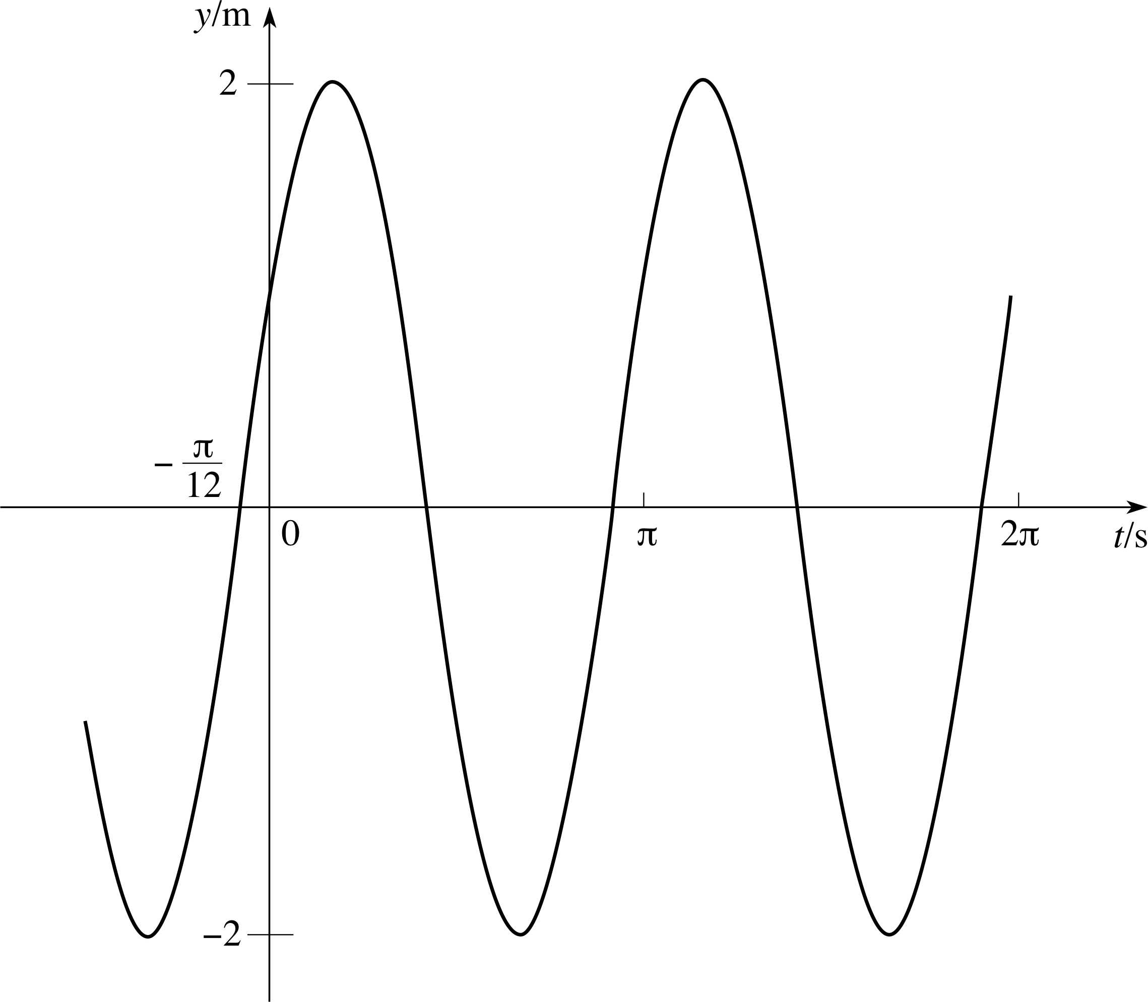
Figure 3 A sinusoidal curve with period π s−1, amplitude 2 m and phase constant π/6.
Equation 19 shows us that, for any particular choice of the constants A and ϕ, the graph of the solution to Equation 15 always has the shape of a sine curve (though it may not pass through the origin). Such a curve is called sinusoidal; an example is shown in Figure 3. We can also deduce from Equation 19 that, since the maximum value attained by a sine function is 1, the maximum value of y is equal to the constant A; therefore A is the amplitude of the oscillations. The other constant ϕ is known as the phase constant or initial phase of the oscillations. Clearly the value of y at t = 0 depends on both A and ϕ since it is equal to A sin ϕ. Thus, if we know the value of ω0, and we can discover the values of A and ϕ (so that we are dealing with a particular solution of Equation 15) we can easily use Equation 19 to construct the graph of the solution. i
The example shown in Figure 3 corresponds to the values A = 2 m, ϕ = π/6 and ω0 = 2 s−1, so that y = (2 m) sin[(2 s−1)t + π/6]. (Notice that y = 0 when t = −(π/12) s, and y = 1 m when t = 0).
Converting from one form of the solution into the other
It is clearly important to be able to switch between the two forms of the solution to the SHM equation given in Equations 16 and 19.
From Equations 17a and b we can easily calculate B and C if we are given values for A and ϕ; but how do we calculate A and ϕ from known values of B and C? To see how to do this, note that if
B = A sin ϕ and C = A cos ϕ(Eqns 17a, b)
then
B2 + C 2 = A2 (sin2ϕ +cos2ϕ) = A2
so that
A2 = B2 + C 2
By convention, A is always taken to be positive, so we have the following two equations for A and ϕ, where Equation 21 is obtained from Equations 17a and b by dividing the expression for B by the expression for C. i
Equations converting from the first form of the solution of the SHM equation into the second form:
$A = \sqrt{B^2 + C^2}$ (positive square root)(20)
$\dfrac BC = \dfrac{A\sin\varphi}{B\cos\varphi} = \tan\varphi$ i.e. ϕ = arctan(B/C) but with 0 ≤ ϕ < 2π(21)
By convention, ϕ is always chosen to lie within the range 0 ≤ ϕ < 2π in this context. You may be wondering why it cannot be chosen to lie within the range −π/2 ≤ ϕ < π/2 – the standard range for the inverse tan function – the reason is that although the function tan ϕ repeats itself as ϕ is increased by π, sin ϕ and cos ϕ do not. Thus the range −π/2 ≤ ϕ < π/2 would not cover all possible values (both positive and negative) of the constants B and C.
In fact, using Equation 17 and our knowledge of the properties of sin ϕ and cos ϕ, we can lay down some rules for the range of values within which ϕ must lie, depending on whether B and C are positive or negative:
B ≥ 0 and C ≥ 0 ⇒ 0 ≤ ϕ ≤ π/2(22a) i
B ≥ 0 and C < 0 ⇒ π/2 < ϕ ≤ π(22b)
B < 0 and C < 0 ⇒ π < ϕ < 3π/2(22c)
B < 0 and C ≥ 0 ⇒ 3π/2 ≤ ϕ < 2π(22d)
You can now use Equations 17, 20, 21 and 22 to answer the following questions:
Question T5
Write the particular solution y = 6 sin(3t + π/3) in the form y = B cos(ω0t) + C sin(ω0t).
Answer T5
The solution is given in the form y = Asin(ω0t + ϕ), where A = 6, ϕ = π/3 and ω0 = 3. Using Equation 17,
B = A sin ϕ and C = A cos ϕ(Eqns 17a, b)
we find that $B = A\sin\varphi = 6\sin(\pi/3) = 6 \times \sqrt{3\os}/2 \approx 5.20$ and C = A cos ϕ = 6 cos(π/3) = 3. So this particular solution may be written as y = 5.20 cos(3t) + 3 sin(3t).
Question T6
Write the two following particular solutions in the form y = Asin(ω0t + ϕ):
(a) y = 4 cos(2t) + 3 sin(2t) (b) y = 5 sin(4t) − 12 cos(4t)
Answer T6
These solutions are both of the form
y = B cos(ω0t) + Csin(ω0t)
(a) Here B = 4, C = 3, ω0 = 2. From Equation 20,
$A = \sqrt{B^2+C^2}$ (positive square root)(Eqn 20)
$A = \sqrt{3^2+4^2} = 5$ (remember that by convention A is positive), and from Equation 21,
$\dfrac BC = \dfrac{A\sin\varphi}{B\cos\varphi} = \tan\varphi$ i.e. ϕ = arctan(B/C) but with 0 ≤ ϕ < 2π(Eqn 21)
ϕ = arctan(4/3), which has two values: 0.927 or π + 0.927. Looking at Equation 22a,
B ≥ 0 and C ≥ 0 ⇒ 0 ≤ ϕ ≤ π/2(Eqn 22a)
we see that since both B and C are positive, 0 < ϕ < π/2; so ϕ = 0.927. So this solution can be written as
y = 5 sin(2t + 0.927)
(b) Here B = −12, C = 5, ω0 = 4. From Equation 20,
$A = \sqrt{(-12)^2+5^2} = 13$
and from Equation 21,
ϕ = arctan(−12/5), which has two values: 1.966 or π + 1.966. Looking at Equation 22d,
B < 0 and C ≥ 0 ⇒ 3π/2 ≤ ϕ < 2π(Eqn 22d)
we see that since B is negative and C is positive, 3π/2 ≤ ϕ < 2π; so ϕ = π + 1.966 = 5.108. So this solution can be written as
y = 13 sin(4t + 5.108).
2.4 Equations of the form d2y/dt2 − λ2y = 0
We will now return to the case of negative h in Equation 14.
$\dfrac{d^2y}{dt^2} + hy = 0$(Eqn 14)
If h is negative, we can make it clear that this is so by writing h = −λ2, where (by convention) λ > 0, so that Equation 14 becomes
$\dfrac{d^2y}{dt^2} - \lambda^2y = 0$(23) i
You may not have yet encountered any physical situations that could be described by an equation of this sort. However, it does have important applications in quantum physics and elsewhere. So it is well worth your while to learn how to solve this equation. Moreover, the solution is very easy to find.
To solve Equation 23, let us proceed using the same sort of informed guesswork that we used to solve Equation 15.
$\dfrac{d^2y}{dt^2} + \omega_0^2 y = 0$(Eqn 15)
In the case of Equation 15, we wanted to find a function such that its second derivative was equal to the function itself multiplied by a negative constant. Looking at Equation 23, we see that this time we want a function (or functions) the second derivative of which is equal to the function itself multiplied by a positive constant. Exponential functions have the property that all their derivatives are proportional to the function itself.
So let us see if an exponential function, of the form
y = Bept(24)
where B is an arbitrary constant, is a solution of Equation 23.
If we differentiate Equation 24 once we find
$\dfrac{dy}{dt} = pB{\rm e}^{pt} = py$
When we differentiate again, we find
$\dfrac{d^2y}{dt^2} = p\dfrac{dy}{dt} = p^2y$
and on substituting this result into Equation 23 we obtain
p2y − λ2y = 0
which is an identity i provided that p2 = λ2. Thus Equation 24 is a solution to Equation 23 provided p = +λ or p = −λ.
It follows that any function of the form
y = Beλt(25a)
ory = Ce−λt(25b)
(We have replaced the arbitrary constant B in Equation 25a by the arbitrary constant C in Equation 25b.)
is a solution to Equation 23.
Neither of these equations can themselves be the general solution of Equation 23, as neither contains two arbitrary constants. But perhaps their sum, which does contain two arbitrary constants, is the general solution.
✦ Show that y = Beλt + Ce−λt is a solution to Equation 23.
✧
$\dfrac{dy}{dt} = \lambda B{\rm e}^{\lambda t} - \lambda C{\rm e}^{-\lambda t}$,
and$\dfrac{d^2y}{dt^2} = \lambda^2 B{\rm e}^{\lambda t} + \lambda^2 C{\rm e}^{-\lambda t} = \lambda^2y$
Soλ2y − λ2y = 0
So this function is indeed a solution.
Alternatively, we could show that if y1 and y2 are both solutions then y = (y1 + y2) must be a solution because
y′′ = (y1 + y2)′′ = y1′′ + y2′′ = λ2y1 + λ2y2 = λ2(y1 + y2) = λ2y
So you have shown that:
The general solution of Equation 23 is
y (t) = Beλt + Ce−λt(26)
Since Equation 26 contains two arbitrary constants, it is the general solution. You may wonder what this solution looks like graphically. If either B or C is zero, the curve is exponential. Otherwise, the solution given in Equation 26 behaves like y = B exp(λt) when t is large and positive (as then exp(−λt) is very small), and like y = C exp(−λt) when t is large and negative (as then exp(λt) is very small). Figure 4 shows the four general shapes of curve you can expect, depending on the different signs of B and C.
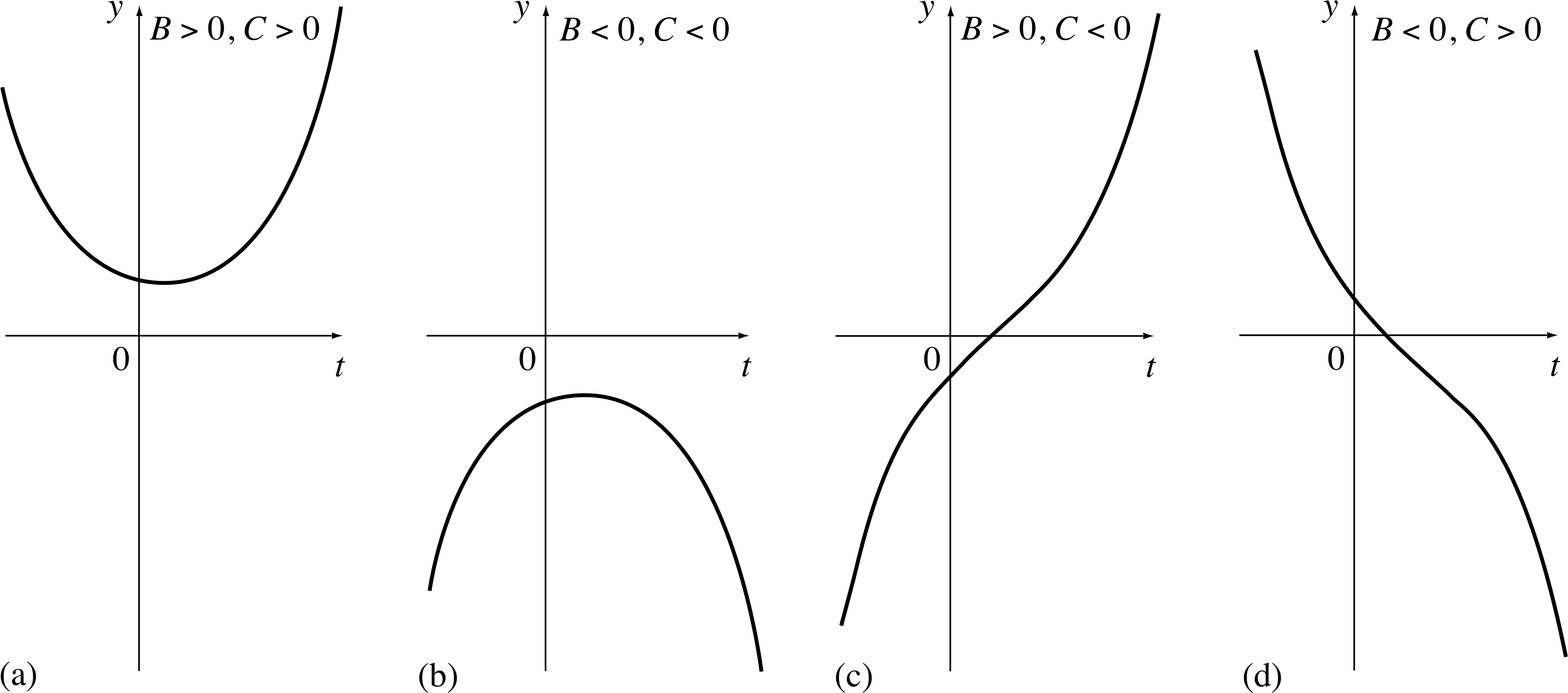
Figure 4 Solutions to Equation 23. General solution is y (t) = Beλt + Ce−λ
Question T7
Find the general solution of
$\dfrac{d^2y}{dx^2} - 4y = 0$
and the particular solution if y = 6 and dy/dx = 0 at x = 0.
Answer T7
Here λ2 = 4. So from Equation 26,
y (t) = Beλt + C e−λt(Eqn 26)
the general solution is
y = Be2t − Ce−2t
Hence$\dfrac{dy}{dx} = 2B{\rm e}^{2x} - 2C{\rm e}^{-2x}$
If we substitute the initial values of y and dy/dx into these equations we find 6 = B + C and 0 = 2B − 2C, from which it follows that B = C = 3. So the particular solution is y = 3e2t + 3 e−2t.
We obtained the general solution given in Equation 26 by taking the sum of the two solutions given in Equation 25. In fact, it can be proved that, for any linear homogeneous equation (not necessarily one with constant coefficients) the sum of two solutions (or more than two, if the equation is of higher order than the second) is always also a solution. We will not give the proof here (although the answer to the P2-questionlast Seed Question should provide a hint as to how the proof might go), but you should bear this useful result in mind; we will make use of it in the next subsection.
2.5 The equation for damped harmonic motion: a (d2y/dt2) + b (dy/dt) + cy = 0
In Subsection 2.3, we mentioned that an equation of the form
$a\dfrac{d^2y}{dt^2} + cy = 0$ where c/a = h > 0
has many different applications in physics, describing, as it does, the behaviour of an object undergoing simple harmonic motion. Its solutions are sinusoidal oscillations of constant amplitude. However, you know from experience that the vibrations of an oscillating object always die away with time (pendulum clocks run down; masses bobbing up and down on springs come to rest, and so on). This is due to the effect of resistive or damping forces, which oppose the motion of the oscillating object. How can we modify the SHM equation (Equation 15).
$\dfrac{d^2y}{dt^2} + \omega+0^2 y = 0$(Eqn 15)
to take account of these forces? Let us return to the example mentioned in Subsection 1.1, a mass m oscillating up and down on a spring of force constant k.
If the restoring force of the spring, −ky, is the only force acting on the mass, then, according to Newton’s second law, its displacement y (t) must satisfy the equation
$m\dfrac{d^2y}{dt^2} = -ky$
To incorporate the effects of a damping force, we must add a term on the right–hand side which always acts in a direction opposite to the direction of the velocity of the mass (the bob). A simple way of doing this is to assume that the damping force can be written in the form −b (dy/dt), where b is a positive constant, so that the equation of motion of the mass becomes
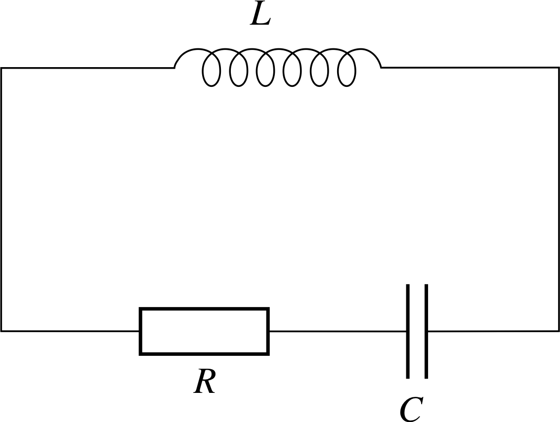
Figure 5 A circuit containing an inductance L, a resistor R and a capacitor C, connected in series.
$m\dfrac{d^2y}{dt^2} = -ky - b\dfrac{dy}{dt}$ i
i.e.$m\dfrac{d^2y}{dt^2} + b\dfrac{dy}{dt} + ky = 0$(27)
An equation of the form given in Equation 27 also arises in the theory of a.c. circuits.
The current I in the circuit shown in Figure 5, containing an inductance L, a resistor R and a capacitor C, obeys the differential equation
$L\dfrac{d^2I}{dt^2} + R\dfrac{dI}{dt} + \dfrac IC = 0$(28)
To predict the behaviour of the mass on the spring, or the current in the circuit, you need to be able to solve differential equations of the type
$a\dfrac{d^2y}{dt^2} + b\dfrac{dy}{dt} + cy = 0$ where a > 0, b > 0 and c > 0(29) i
We need the ratio b/a to be positive if the coefficient of dy/dt is to represent a resistive force, opposing the velocity of the object; and we need the ratio c/a to be positive so that if b is zero, we recover the SHM equation (Equation 15).
$\dfrac{d^2y}{dt^2} + \omega+0^2 y = 0$(Eqn 15)
This condition is most simply achieved by restricting all three constants to positive values. (In fact, the solutions we obtain to Equation 29 will apply equally well if any of a, b, or c is negative.)
Let us now try to find solutions to Equation 29.
We know that if b = 0, then the solution is a sinusoidal function. However, we do not want a purely sinusoidal solution if b > 0 (we want y to tend to zero as t becomes large and positive, due to the damping); moreover, if you try a solution of the form y = sin(pt) or cos(pt) in Equation 29, you will quickly find that it does not work (unless b = 0, of course). But perhaps an exponential function would work, just as it did for Equation 23?
$\dfrac{d^2y}{dt^2} - \lambda^2y = 0$(Eqn 23)
We have nothing to lose by trying it, so let us substitute
y = Bept(30)
into Equation 29.
The first derivative of y is equal to py, and the second derivative is equal to p2y; so we find, on substitution,
ap2y + bpy + cy = 0
which is an identity provided that p satisfies the equation
ap2 + bp + c = 0 (auxilliary equation)(31)
This quadratic equation in p is known as the auxiliary equation of Equation 29.
As it is a quadratic, the roots of Equation 31 are given by i
$p_1 = \dfrac{-b+\sqrt{b^2-4ac}}{2a}\quad\text{and}\quad p_2 = \dfrac{-b-\sqrt{b^2-4ac}}{2a}$(32)
This formula will give us two real values for p1 and p2 provided that b2 > 4ac. (We will deal with the cases where b2 < 4ac or b2 = 4ac shortly; but for the moment, let us assume that the two roots are real.)
We have shown, therefore, that the trial solution, Equation 30, will satisfy Equation 29 for any value of B provided that p is one of the two roots given in Equation 32.
Real roots of the auxiliary equation (heavy damping)
We can write the two solutions of Equation 29,
$a\dfrac{d^2y}{dt^2} + b\dfrac{dy}{dt} + cy = 0$ where a > 0, b > 0 and c > 0(Eqn 29)
we have just found as
y = B exp(p1t) and y = C exp(p2t)
As we mentioned at the end of Subsection 2.4, we can obtain the general solution to Equation 29 by adding these two solutions together:
The general solution of Equation 29 in the case b2 > 4ac is
y (t) = B exp(p1t) + C exp(p2t)(33)
where$p_1 = \dfrac{-b+\sqrt{b^2-4ac}}{2a}\quad\text{and}\quad p_2 = \dfrac{-b-\sqrt{b^2-4ac}}{2a}$
or, written out in full,
$y = B\exp\left(\dfrac{-b+\sqrt{b^2-4ac}}{2a}\right) + C\exp\left(\dfrac{-b-\sqrt{b^2-4ac}}{2a}\right)$(34)
There is no need to memorize this unpleasant–looking equation – but you should remember the method that we used to derive it, and be able to apply it to a given differential equation, as in the following example.
Example 2
Find the general solution of the differential equation
$\dfrac{d^2y}{dt^2} + 5\dfrac{dy}{dt} + 6y = 0$
Solution
First write down the auxiliary equation,
p2 + 5p + 6 = 0
This equation has two real roots:
$p = -\frac52 \pm \frac12\sqrt{25 - 24\os}$ = −2 or −3 i
Thus the general solution is y = Be−2t + Ce−3t.
Question T8
Find the general solution of the differential equation
$6\dfrac{d^2y}{dt^2} + 17\dfrac{dy}{dt} + 12y = 0$
Answer T8
The auxiliary equation is 6p2 + 17p + 12 = 0. This equation has the real roots
$p = \dfrac{-17 \pm \sqrt{289 - 288\os}}{12} = -\dfrac 43 \text{ or } -\dfrac32$
So the general solution is y = B exp(−4t/3) + C exp(−3t/2).
You can see that if a, b and c are all positive quantities, the positive square root $\sqrt{b^2-4ac}$ must be less than b, and therefore both roots of the auxiliary equation are negative. Thus the solution to Equation 29,
$a\dfrac{d^2y}{dt^2} + b\dfrac{dy}{dt} + cy = 0$ where a > 0, b > 0 and c > 0(Eqn 29)
that is given in Equation 34,
$y = B\exp\left(\dfrac{-b+\sqrt{b^2-4ac}}{2a}\right) + C\exp\left(\dfrac{-b-\sqrt{b^2-4ac}}{2a}\right)$(Eqn 34)
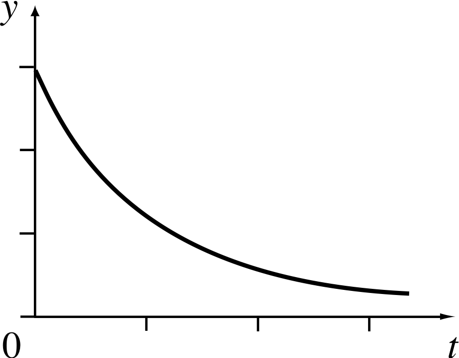
Figure 6 Heavily damped motion.
is the sum of two decreasing exponentials, and as t becomes very large and positive, y tends to zero. An example of this is shown in Figure 6.
Remember that in physical situations b gives an indication of the magnitude of the damping force. If b = 0 the motion is dampingundamped and we have oscillations corresponding to SHM (as in Equation 15),
$\dfrac{d^2y}{dt^2} + \omega_0^2 y = 0$(Eqn 15)
but if b is so large that b2 > 4ac, then there are no oscillations (as in Figure 6). In such a case, the motion is said to be heavily damped. You can probably guess what will happen if we choose a value for b somewhere between these two extremes. Nonetheless, we will now analyse such problems systematically.
Complex roots of the auxiliary equation (light damping)
We will now solve Equation 29,
$a\dfrac{d^2y}{dt^2} + b\dfrac{dy}{dt} + cy = 0$ where a > 0, b > 0 and c > 0(Eqn 29)
for the case b2 < 4ac. We will give two alternative treatments of this important case.
The first treatment depends on a result that comes from the study of complex numbers, and shows that the solution in this case is merely an extension of the previous result.
The second treatment does not require as much knowledge of complex numbers, we will just give you the solution of the differential equation and ask you to verify that what we say is correct.
The first treatment requires the following result from the theory of complex numbers
eiθ = cos θ + i sin θ(35) i
If you are familiar with this result continue reading; if not go straight to Question T9.
If b2 < 4ac in Equation 29, then the two roots of Equation 31,
ap2 + bp + c = 0 (auxilliary equation)(Eqn 31)
are complex and can be written (using Equation 32)
$p_1 = \dfrac{-b+\sqrt{b^2-4ac}}{2a}\quad\text{and}\quad p_2 = \dfrac{-b-\sqrt{b^2-4ac}}{2a}$(Eqn 32)
as $p_1 = -\dfrac{\gamma}{2} + i \dfrac{\omega}{2}\quad\text{and}\quad p_1 = -\dfrac{\gamma}{2} - i \dfrac{\omega}{2}$ i
where γ = b/a and $\omega = \sqrt{4ac-b^2}/(2a)$ (Notice that, since b2 < 4ac, we can be sure that ω is a real quantity.) i
Thus, the general solution to Equation 29 when b2 < 4ac is similar to that given in Equation 33,
y (t) = B exp(p1t) + C exp(p2t)(Eqn 33)
and we may write it as
$y = R\exp\left[\left(-\dfrac{\gamma}{2} + i \dfrac{\omega}{2}\right)t\right] + S\exp\left[\left(-\dfrac{\gamma}{2} - i \dfrac{\omega}{2}\right)t\right] = \exp(-\gamma t/2)\left[R\exp(i\omega t)+S\exp(-i\omega t)\right]$(36)
where R and S are arbitrary constants.
It looks as though this solution will give complex values to y. However, since the case b2 < 4ac frequently arises in physics problems, it must be possible to arrange Equation 36 in a form which need not involve any complex quantities. We do this by employing Equation 35,
eiθ = cos θ + i sin θ(Eqn 35)
to write
exp(iωt) = cos(ωt) + i sin(ωt) and exp(−iωt) = cos(ωt) − i sin(ωt)
If we substitute these results into Equation 36, we find
y = exp(γt/2)[(R + S) cos(ωt) + i (R − S) sin(ωt)]
We can now define new arbitrary constants B = R + S and C = i (R − S), and rewrite the solution as
y = exp(−γt/2)[B cos(ωt) + C sin(ωt)]
You may think that this rewriting has achieved nothing since C may be complex, so we have still not ensured that the solution y (t) is a real quantity. However, at this point it is important to realize that the constants R and S in Equation 36 are quite arbitrary, they did not even have to be real. Equation 36 is a perfectly valid solution to Equation 29,
$a\dfrac{d^2y}{dt^2} + b\dfrac{dy}{dt} + cy = 0$ where a > 0, b > 0 and c > 0(Eqn 29)
even if R and S are complex. In fact, if R and S are complex conjugates, i.e. complex numbers of the form
R = a + ib and S = a − ib where a and b are real constants
then B = R + S = 2a will be real
andC = i (R − S) = i (2ib) = −2b will be real
Moreover, the values of a and b are unrelated, so we are free to choose arbitrary values for the constants B and C just as we were for R and S.
Thus:
The general solution of Equation 29 in the case b2 < 4ac is
y (t) = exp(−γt/2)[(B cos(ωt) + C sin(ωt)](37)
withγ = b/a(38a)
and$\omega = \sqrt{4ac-b^2}{\large/}(2a)$(38b)
Question T9
Show by substitution that, for arbitrary constants B and C
y (t) = exp(−γt/2)[B cos(ωt) + C sin(ωt)]
where γ = b/a and $\omega = \sqrt{4ac-b^2}{\large/}(2a)$
is a solution to Equation 29.
$a\dfrac{d^2y}{dt^2} + b\dfrac{dy}{dt} + cy = 0$ where a > 0, b > 0 and c > 0(Eqn 29)
(Notice that ω is a real quantity if b2 < 4ac.)
Answer T9
Two methods of solution are given in this answer; the first is straightforward but laborious, the second is shorter.
Method 1 If y = exp(−γt/2)[B cos(ωt) + C sin(ωt)] then
$\dfrac{dy}{dt} = \exp\left(-\dfrac{\gamma t}{2}\right)\left[\left(-\dfrac{\gamma B}{2}+\omega C\right)\cos(\omega t) + \left(-\dfrac{\gamma C}{2}-\omega B\right)\sin(\omega t)\right]$
and
$\dfrac{d^2y}{dt^2} = \exp\left(-\dfrac{\gamma t}{2}\right)\left[\left(\dfrac{\gamma^2 B}{2}-\gamma\omega C-\omega^2B\right)\cos(\omega t) + \left(\dfrac{\gamma^2 C}{2}+\gamma\omega B-\omega^2C\right)\sin(\omega t)\right]$
The easiest way to proceed is to substitute these expressions into the left–hand side of Equation 29,
$a\dfrac{d^2y}{dx^2} + b\dfrac{dy}{dx} + cy = 0$ where a > 0, b > 0 and c > 0(Eqn 29)
collect together similar terms B exp(−γt/2) cos(ωt), B exp(−γt/2) sin(ωt), and so on, and then look at their coefficients. For example, we find that the coefficient of B exp(−γt/2) cos(ωt) is
a (γ2 − ω2) − bγ/2 + c = a (b2/2a2 − c/a) + b (−b/2a) + c = 0
on using Equation 38,
γ = b/2 and $\omega = \sqrt{4ac-b^2}/(2a)$(Eqn 38a and b)
The coefficient of C exp(−γt/2) cos(ωt) is (−aγω + bω), which clearly vanishes since γ = b/a. The coefficients of C exp(−γt/2) cos(ωt) and C exp(−γt/2) sin(ωt) can also be shown to vanish using Equation 38. Thus the left–hand side is identically equal to zero, and so Equation 37 gives a solution,
y (t) = exp(−γt/2)[(B cos(ωt) + C sin(ωt)](Eqn 37)
Comment If you managed to do the question this way, congratulations! The algebra is quite unpleasant. Read on for a second method.
Method 2 Proceed as before by writing y = exp(−γt/2)[B cos(ωt) + C sin(ωt)]
then use the abbreviations y′ and y′′ (to save work) and write
$y' = -\dfrac{\gamma}{2}\exp(-\gamma t/2)[B\cos(\omega t) + C\sin(\omega t)] + \exp(-\gamma t/2)[-B\omega\sin(\omega t) + C\omega\cos(\omega t)]$
$\phantom{y' }= -\dfrac{\gamma}{2}y + \exp(-\gamma t/2)[-B\omega\sin(\omega t) + C\omega\cos(\omega t)]$
Now differentiate again to find
$y'' = -\dfrac{\gamma}{2}y' - \dfrac{\gamma}{2}\left\{\exp(-\gamma t/2)[-B\omega\sin(\omega t) + C\omega\cos(\omega t)] + \exp(-\gamma t/2)[-B\omega\cos(\omega t) - C\omega\sin(\omega t)\right]$
$\phantom{y'' }= -\dfrac{\gamma}{2}y' - \dfrac{\gamma}{2}\left(y' + \dfrac{\gamma}{2}y\right) - \omega^2 y$
which can be rearranged to give
$y'' + \gamma y' + \left(\dfrac{\gamma^2}{4} + \omega^2\right)y = 0$
Using the fact that
$\omega = \sqrt{4ac-b^2}/(2a)$ and γ = b/a
this reduces to the original equation ay′′ + by′ + cy = 0.
(If you favour this method you will have an opportunity to try it in Question T10).
The combination [B cos(ωt) + C sin(ωt)] appears in Equation 37, and it may be convenient to write this instead in the form A sin(ωt + ϕ), as we did in Subsection 2.3, by putting
$A = \sqrt{B^2 + C^2}$ (positive square root)(Eqn 20)
$\dfrac BC = \dfrac{A\sin\varphi}{B\cos\varphi} = \tan\varphi$ i.e. ϕ = arctan(B/C) but with 0 ≤ ϕ < 2π(Eqn 21) i
This gives:
The alternative form of the solution of Equation 29 in the case b2 < 4ac
y (t) = A exp(−γt/2) sin(ωt + ϕ)(39)
with γ = b/2 and $\omega = \sqrt{4ac-b^2}/(2a)$(Eqn 38a and b)
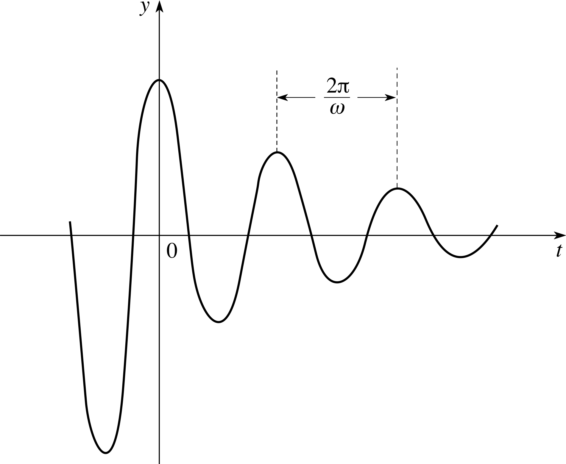
Figure 7 Lightly damped oscillations.
From Equation 39 it is easy to determine the behaviour of the function y (t). Since b/a is positive, γ is also positive – so y (t) is given by a sinusoidal function multiplied by an exponential function that decays as t becomes large and positive.
Figure 7 shows the form of the solution in this case. You can see that the effect of multiplying the sinusoidal function by the exponential is to produce oscillations with amplitudes that decrease with time.
This is just the sort of behaviour we expect of a system where the resistive forces are not too large – remember that b2 must be less than 4ac for the solution in Equation 39 to apply.
In this case, the system is said to be lightly damped. Note that the values of t for which y = 0 are still equally spaced, with separation, ∆t say, given by ω∆t = π, or ∆ t = π/ω. Successive maxima and minima are also equally spaced, by an interval in t equal to 2π/ω (though they no longer occur exactly half–way between the points where y = 0).
For these reasons, we still speak of the quantity 2π/ω as the period of the oscillations.
Equal roots of the auxiliary equation (critical damping)
Finally, we will consider the case where b2 = 4ac which (although it is somewhat artificial in that it rarely occurs in practice) is of interest because it marks the transition from light to heavy damping. In this case, the auxiliary Equation 31,
ap2 + bp + c = 0 (auxilliary equation)(Eqn 31)
has only one root; from Equation 32,
$p_1 = \dfrac{-b+\sqrt{b^2-4ac}}{2a}\quad\text{and}\quad p_2 = \dfrac{-b-\sqrt{b^2-4ac}}{2a}$(Eqn 32)
we see that p1 = p2 = −b/(2a). We deduce that y = B exp[−bt/(2a)] is a solution of the differential equation Equation 29.
$a\dfrac{d^2y}{dt^2} + b\dfrac{dy}{dt} + cy = 0$ where a > 0, b > 0 and c > 0(Eqn 29)
However, it cannot be the general solution, since it only contains one arbitrary constant. The other solution that we must add to it is not at all obvious, so we will just tell you the answer, and leave you to check it by substitution:
The general solution of Equation 29 in the case b2 = 4ac is
y (t) = (B + Ct) exp[−bt/(2a)](40)
Question T10
Show that Equation 40 is a general solution of Equation 29 in the case b2 = 4ac.
Answer T10
To save work we will introduce the notation p = −b/(2a), so that the trial solution (Equation 40)
y (t) = (B + Ct) exp[−bt/(2a)](Eqn 40)
is y = (B + Ct)ept. Therefore
$\dfrac{dy}{dt} = (pCt + pB + C){\rm e}^{pt}$
and$\dfrac{d^2y}{dt^2} = (p^2Ct + p^2B + 2pC){\rm e}^{pt}$
We now substitute these expressions into Equation 29,
$a\dfrac{d^2y}{dt^2} + b\dfrac{dy}{dt} + cy = 0$(Eqn 29)
collect together terms in t exp(pt) and exp(pt), and check whether their coefficients vanish, using the relations
p = −b/(2a) and b2 − 4ac = 0.
The coefficient of t exp(pt) is ap2C + bpC + cC = (b2/4a − b2/2a + c)C = 0 and the coefficient of exp(pt) is a (p2B + 2pC) + b (C + pB) + cB = C (−b + b) + B (b2/4a − b2/2a + c) = 0
So the left–hand side is identically equal to zero, and hence Equation 40 is a solution.
Alternatively, we can write y = (B + Ct)ept so that
y′ = Cept + py
andy′′ = pCept + py′
y′′ = p (y′− py) + py′ (because Cept = y′− py)
y′′ = 2py′ − p2y
which can be rearranged to give y′′ − 2py′ + p2y = 0, which becomes ay′′ + by′ + cy = 0 (using p = −b/(2a) and b2 − 4ac = 0).
This has been a long and quite complicated subsection, which is perhaps misleading since in practice the solution of Equation 29 is fairly straightforward, and just a matter of knowing how to deal with three cases. Here then is a summary of the steps you need to follow in order to solve the equation of damped harmonic motion:
$a\dfrac{d^2y}{dt^2} + b\dfrac{dy}{dt} + cy = 0$ where a > 0, b > 0 and c > 0(Eqn 29)
- Step 1
-
Evaluate the quantity b2 − 4ac
- Step 2
-
If b2 > 4ac:
Find the roots p1 and p2 of the auxiliary equation, Equation 31,
ap2 + bp + c = 0 (auxilliary equation)(Eqn 31)
The general solution is then given by Equation 33,
y (t) = B exp(p1t) + C exp(p2t)(Eqn 33)
If b2 < 4ac:
Find the quantities γ and ω, using Equation 38,
withγ = b/a(Eqn 38a)
and$\omega = \sqrt{4ac-b^2}$(Eqn 38b)
The general solution is then given by Equation 37,
y (t) = exp(−γt/2)[(B cos(ωt) + C sin(ωt)](Eqn 37)
Use Equations 20 and 21,
$A = \sqrt{B^2+C^2}$(Eqn 20)
ϕ = arctan(B/C) but with 0 ≤ ϕ < 2π(Eqn 21)
if you want the solution in the form of Equation 39,
y (t) = A exp(−γt/2) sin(ωt + ϕ)(Eqn 39)
If b2 = 4ac:
The general solution is given by Equation 40,
y (t) = (B + Ct) exp[−bt/(2a)](Eqn 40)
Now practise these steps by trying the following question. You must make sure that you have mastered the techniques required in these exercises. You will not be able to make progress with the next section unless you have done so.
Question T11
Find the general solution of each of the following differential equations:
(a) $\dfrac{d^2x}{dt^2} + 6\dfrac{dx}{dt} + 10x = 0$ (b) $2\dfrac{d^2y}{dx^2} + 5\dfrac{dy}{dx} + 3y = 0$ (c) $5\dfrac{d^2y}{dt^2} + 6\dfrac{dy}{dt} + 2y = 0$ (d) $\dfrac{d^2y}{dt^2} + 2\dfrac{dy}{dt} + y = 0$
Answer T11
(a) Step 1 Here a = 1, b = 6, c = 10. So b2 − 4ac = 36 − 40 = −4.
Step 2 Since b2 − 4 ac < 0, the general solution is of the form given in Equation 37 (or Equation 39),
y (t) = exp(−γt/2)[(B cos(ωt) + C sin(ωt)](Eqn 37)
y (t) = A exp(−γt/2) sin(ωt + ϕ)(Eqn 39)
Here γ = b/a = 6, $\omega = \sqrt{4ac-b^2}/(2a) = 1$ so the general solution is
x = exp(−3t)(B cos t + C sin t)
(b) Step 1 Here a = 2, b = 5, c = 3. So b2 − 4ac = 25 − 24 = 1.
Step2 Since b2 −4ac > 0, we find the roots of the auxiliary equation, 2p2 + 5p + 3 = 0. These are p1 = −1 and p2 = −3/2 so the general solution, given by Equation 33,
y (t) = B exp(p1t) + C exp(p2t)(Eqn 33)
isy = B exp(−x) + C exp(−3x/2)
(Note the change of independent variable from t to x.)
(c) Step 1 Here a = 5, b = 6, c = 2. So b2 − 4ac = 36 − 40 = −4.
Step 2 Since b2 − 4ac < 0, the general solution is of the form given in Equation 37 (or Equation 39),
y (t) = exp(−γt/2)[(B cos(ωt) + C sin(ωt)](Eqn 37)
y (t) = A exp(−γt/2) sin(ωt + ϕ)(Eqn 39)
Here, γ = b/a = 1.2 and $\omega = \sqrt{4ac-b^2}/(2a) = 0.2$
So the general solution is
y = exp(−0.6t)[B cos(0.2t) + C sin(0.2t)]
(d) Step 1 Here a = 1, b = 2 and c = 1, so that b2 − 4ac = 4 − 4 = 0.
Step 2 Since b2 − 4ac = 0 the general solution is of the form given in Equation 40,
y (t) = (B + Ct) exp[−bt/(2a)](Eqn 40)
withb/(2a) = 1 so y = (B + Ct) exp(−t).
The method of comparing b2 with 4ac and then selecting the form of the solution will of course work even if b = 0, that is, for the differential equations discussed in Subsection 2.3Subsections 2.3 and Subsection 2.42.4. Consider, for example,
$\dfrac{d^2y}{dt^2} + \omega_0^2 y = 0$(Eqn 15) i
Here, b = 0, a = 1 and c = ω02. So b2 < 4ac, and Equation 38,
γ = b/a(Eqn 38a)
$\omega = \sqrt{4ac-b^2}$(Eqn 38b)
tells us that γ = 0, ω = ω0. Thus using Equation 37,
y (t) = exp(−γt/2)[(B cos(ωt) + C sin(ωt)](Eqn 37)
we see that the general solution is y (t) = B cos(ω0t) + C sin(ω0t), which is just what we found before, in Equation 16.
y (t) = B cos(ω0t) + C sin(ω0t)(Eqn 16)
2.6 Equations of the form a (d2y/dt2) + b (dy/dt) + cy = f (t)
We are now in a position to set about finding solutions to the general second–order linear inhomogeneous
equation with constant coefficients:
$a\dfrac{d^2y}{dt^2} + b\dfrac{dy}{dt} + cy = f(t)$(Eqn 5)
We will first of all show that if we can find any one particular solution to Equation 5, then we can always find the general solution. We will then show a method that can sometimes be used to find particular solutions.
Let us suppose that we have somehow managed to find a particular solution to Equation 5; we will call it yp(t). We now assert that the general solution is obtained by taking the sum of yp(t) and the general solution to the homogeneous equation which is obtained by setting f (t) = 0 in Equation 5:
$a\dfrac{d^2y}{dt^2} + b\dfrac{dy}{dt} + cy = 0$(41)
In this context, the general solution to the homogeneous equation (Equation 14)
$\dfrac{d^2y}{dt^2} + hy = 0$(Eqn 14)
is called the complementary function; we will denote it by yc(t). Thus the claim here is that the general solution to Equation 5 is
y (t) = yp(t) + yc(t)(42)
This result is easy to prove. We simply substitute Equation 42 into Equation 5. The left–hand side becomes
$a\dfrac{d^2}{dt^2}(y_{\rm p} + y_{\rm c}) + b\dfrac{d}{dt}(y_{\rm p} + y_{\rm c}) + c(y_{\rm p} + y_{\rm c})$
which is equal to
$a\dfrac{d^2y_{\rm p}}{dt^2} + b\dfrac{dy_{\rm p}}{dt} + cy_{\rm p} + a\dfrac{d^2y_{\rm c}}{dt^2} + b\dfrac{dy_{\rm c}}{dt} + cy_{\rm c}$(43)
but by assumption, yp is a solution to Equation 5; that is
$a\dfrac{d^2y_{\rm p}}{dt^2} + b\dfrac{dy_{\rm p}}{dt} + cy_{\rm p} = f(t)$
and yc is the general solution to Equation 41, so that
$a\dfrac{d^2y_{\rm c}}{dt^2} + b\dfrac{dy_{\rm c}}{dt} + cy_{\rm c} = 0$
So we see from Equation 43 that, with the substitution y = yp + yc, the left–hand side of Equation 5 is equal to f (t) + 0, i.e. equal to f (t). Thus Equation 42 is a solution to Equation 5; it is the general solution since yc contains two arbitrary constants.
You should read through the following example carefully because it typifies the method which we apply to all such equations.
Example 3
Find the general solution to the differential equation
$\dfrac{d^2y}{dt^2} + 4y = t$(44) i
given that y = t/4 is a particular solution.
Solution
To find the general solution, we must add the complementary function to the particular solution. The complementary function is the general solution of the homogeneous equation that we obtain by setting the right–hand side of Equation 44 to zero,
$\dfrac{d^2y}{dt^2} + 4y = 0$
This equation is of the form given in Equation 15,
$\dfrac{d^2y}{dt^2} + \omega_0^2y = 0$(Eqn 15)
with ω0 = 2. Its general solution is given by Equation 16,
y (t) = B cos(ω0t) + C sin(ω0t)(Eqn 16)
i.e.B cos(2t) + C sin(2t)
So the general solution to Equation 44 is y = t/4 + B cos(2t) + C sin(2t) i
Question T12
Find the general solution to the differential equation
$\dfrac{d^2y}{dt^2} + 3\dfrac{dy}{dt} - 4y = 2{\rm e}^{-3t}$
given that $y = -\dfrac{{\rm e}^{-3t}}{2}$ is a particular solution.
Answer T12
To find the general solution, we add the complementary function to the particular solution. The complementary function is the general solution of
$\dfrac{d^2y}{dt^2} + 3\dfrac{dy}{dt} - 4y = 0$
which we solve by the method described in Subsection 2.5.
Step 1 Here a = 1, b = 3, c = −4. So b2 − 4ac = 9 + 16 = 25.
Step 2 Since b2 − 4ac > 0, we can find real roots of the auxiliary equation, p2 + 3p − 4 = 0.
These are p1 = 1, p2 = −4, so the complementary function is
Bet + Ce−4t
and hence the general solution to the given equation is
$y = -\frac12{\rm e}^{-3t} + B{\rm e}^t + C{\rm e}^{-4t}$
Finding a particular solution
So we now know how to find a general solution to a linear inhomogeneous equation if we are given a particular solution. But how can we find a particular solution? There are several methods for doing this, and we will explain here only the simplest. It is sometimes known as the method of undetermined coefficients, but as you will see, it consists of little more than intelligent guesswork. The idea is that, guided by the form of f (t), we should assume a particular form for yp(t) which contains some undetermined constants, and simply substitute this into the differential equation. If the form we have chosen is correct, we will be able to determine the constants appearing in our trial solution from the requirement that we must obtain an identity on making the substitution. If we have not chosen the correct form, then we will find that it is not a solution, and we must think again! The method can best be explained by an example.
Example 4
Find a particular solution to the differential equation
$\dfrac{d^2y}{dt^2} + 4\dfrac{dy}{dt} + 5y = t + 2$
Solution
There is a function of the form Ht + K on the right–hand side of this equation. A function of this sort (a polynomial) has the property that when it is differentiated any number of times, no new functions of t appear in its derivatives – indeed, the results are just constants (or zero). This suggests that the differential equation might be satisfied by a function of this sort, with H and K suitably chosen. We may as well try it, anyway.
If we put y = Ht + K into the equation, we obtain
4H + 5 (Ht + K) = t + 2
i.e.5Ht + (4H + 5K) = t + 2
This equation must be an identity if y = Ht + K is a solution. Thus the coefficients of t on both sides must be the same, as must the constant terms. This gives us two equations to be solved for H and K:
5H = 1 and 4H + 5K = 2
These are easily solved, to give H = 1/5, K = 6/25. So we have found a particular solution; it is y = t/5 + 6/25.
If we were to try to generalize the reasoning in Example 4, it would go something like this. The particular solution must be such that when we substitute it into the left–hand side of the equation, f (t) is recovered. If f (t) is a function whose derivatives are all of the same form as f (t) itself (such as a polynomial, an exponential function or a sinusoidal function), we may be able to achieve this by trying as a particular solution a function which is also of the form of f (t), but contains some as yet unknown constants (the ‘undetermined coefficients’), the values of which we will determine when we make the substitution. This leads to the following rules for finding particular solutions, for certain forms of f (t):
Rules for finding particular solutions, for certain forms of f (t):
- 1
-
If f (t) is a polynomial of degree m: try a particular solution that is also a polynomial of degree m
yp(t) = Ht m + Kt m−1 + ... + N
but containing undetermined coefficients H, K ... N
- 2
-
If f (t) is an exponential, Cekt: try a particular solution that is also an exponential,
yp(t) = Hekt
where H is an undetermined coefficient. i
- 3
-
If f (t) is a sinusoidal function, f (t) = Csin(kt) + Dcos(kt): try a particular solution that is also a sinusoidal function
yp(t) = H sin(kt) + K cos(kt)
where H, K are undetermined coefficients.
You can now use Rules 1–3 to answer the following question.
Question T13
Find a particular solution to each of the following equations:
(a) $\dfrac{d^2y}{dx^2} + 2\dfrac{dy}{dx} + 3y = 2{\rm e}^{-x}$ (b) $\dfrac{d^2y}{dx^2} + 4\dfrac{dy}{dx} + 4y = 2\cos x - \sin x$
Answer T13
(a) Since the function on the right–hand side is an exponential, following Rule 2 we will try a particular solution of the same form, H exp(−x), where the coefficient H is to be determined. Substituting this into the equation gives us
He−x − 2He−x + 3He−x = 2e−x
i.e.2He−x = 2e−x which is an identity if H = 1. So y = exp(−x) is a particular solution.
(b) Since the function on the right–hand side is a sinusoidal function, we try a particular solution of the form H cos x + K sin x. Substituting this into the equation gives us
−(H cos x + K sin x) + 4 (−H sin x + K cos x) + 4 (H cos x + K sin x) = 2 cos x − 1 sin x
which is an identity provided that the coefficients of cos x and sin x on each side of the equation are equal. This gives 3H + 4K = 2 and 3K − 4H = −11. Solving these equations gives H = 2, K = −1.
Soy = 2 cos x − sin x is a particular solution.
The method of undetermined coefficients will work for some more complicated forms of f (t), but we have said enough here for you to be able to find particular solutions to many second–order inhomogeneous equations of physical interest. (It is worth pointing out, though, that if f (t) is given by a sum of two or more functions of the sorts mentioned in Rules 1–3, then the particular solution is simply the sum of the particular solutions corresponding to each of these functions.) At the end of the next subsection, in Question T14, you can put together the methods you have learnt so far to find general solutions to inhomogeneous equations. First, however, we will consider an example of great importance in physics.
2.7 A worked example: damped driven harmonic motion
We are now in a position to solve Equation 1, introduced in Subsection 1.1 i
$m\dfrac{d^2y}{dt^2} = -ky - b\dfrac{dy}{dt} + F_0\sin({\it\Omega}t)$(Eqn 1)
rewritten slightly, it is
$m\dfrac{d^2y}{dt^2} + b\dfrac{dy}{dt} + ky = F_0\sin({\it\Omega}t)$(45) i
An equation of this sort applies whenever an oscillating object is subjected to a damping force $\left(-b\dfrac{dy}{dt}\right)$ as well as an external driving force, F0sin(Ωt) with angular frequency Ω. i It is said to describe forced_oscillationsforced, damped oscillations or damped_mechanical_oscillatordamped, driven oscillations.
In this subsection, we will find the general solution to Equation 45 for the case b2 < 4mk.
The complementary function
We will first find the complementary function, i.e. the general solution to
$m\dfrac{d^2y}{dt^2} + b\dfrac{dy}{dt} + ky = 0$
We will solve this using the steps listed at the end of Subsection 2.5. Since we have decided to consider the case b2 < 4mk, the general solution is given by Equation 38,
withγ = b/2 and $\omega = \sqrt{4ac-b^2}/(2a)$(Eqn 38a and b)
with
γ = b/m and $\omega = \sqrt{4mk-b^2}/(2m)$
So the complementary function is
yc(t) = exp[−bt/ (2m)][B cos(ωt) + C sin(ωt)](46)
A particular solution
We will now find a particular solution. We have a sinusoidal function on the right–hand side of Equation 45, so, in accordance with Rule 3 at the end of Subsection 2.6, we will try a particular solution of the form
yp(t) = H cos(Ωt) + K sin(Ωt) i
On substituting this into Equation 45, we find
−mΩ2[H cos(Ωt) + K sin(Ωt)] + bΩ [−H (Ωt) + K cos(Ωt)] + k [H cos(Ωt) + K sin(Ωt)] = F0 sin(Ωt)
which can be rewritten in the form
[(k − mΩ2)H + bΩK] cos(Ωt) + [(k − mΩ2)K − bΩH] sin(Ωt) = F0 sin(Ωt)
If this is to be an identity, the coefficients of cos(Ωt) and sin(Ωt) on each side of the equation must be equal. So we obtain two equations (for H and K)
(k − mΩ2)H + bΩK = 0 and (k − mΩ2)K − bΩH = F0
On solving these equations for H and K, we find (after some algebra! i )
$H = \dfrac{-(b{\it\Omega})F_0}{(k-m{\it\Omega}^2)^2+(b{\it\Omega})^2}\quad\text{and}\quad K = \dfrac{(k-m{\it\Omega}^2)F_0}{(k-m{\it\Omega}^2)^2+(b{\it\Omega})^2}$
Thus the particular solution is the rather complicated looking expression
$y = \dfrac{-(b{\it\Omega})F_0}{(k-m{\it\Omega}^2)^2+(b{\it\Omega})^2}\cos({\it\Omega}t) + \dfrac{(k-m{\it\Omega}^2)F_0}{(k-m{\it\Omega}^2)^2+(b{\it\Omega})^2}\sin({\it\Omega}t)$(47) i
We can simplify this greatly if we use Equations 20 and 21
$A = \sqrt{B^2 + C^2}$ (positive square root)(Eqn 20)
$\dfrac BC = \dfrac{A\sin\varphi}{B\cos\varphi} = \tan\varphi$ i.e. ϕ = arctan(B/C) but with 0 ≤ ϕ < 2π(Eqn 21)
to write yp in the form
yp(t) = A sin(Ωt + ϕ)
Applying Equations 20 and 21, we find (after some more algebra)
$A = \dfrac{F_0}{\sqrt{(k-m{\it\Omega}^2)^2+(b{\it\Omega})^2}}$(48a) i
and$\varphi = \arctan\left(\dfrac{-b{\it\Omega}}{k-m{\it\Omega}^2}\right)$ but with 0 ≤ ϕ ≤ 2π(48b)
The general solution
Thus the general solution of Equation 45,
$m\dfrac{d^2y}{dt^2} + b\dfrac{dy}{dt} + ky = F_0\sin({\it\Omega}t)$(Eqn 45)
given by the sum of the complementary function (Equation 46)
yc(t) = exp[−bt/(2m)][B cos(ωt) + C sin(ωt)](Eqn 46)
and the particular solution (Equation 47),
$y = \dfrac{-(b{\it\Omega})F_0}{(k-m{\it\Omega}^2)^2+(b{\it\Omega})^2}\cos({\it\Omega}t) + \dfrac{(k-m{\it\Omega}^2)F_0}{(k-m{\it\Omega}^2)^2+(b{\it\Omega})^2}\sin({\it\Omega}t)$(Eqn 47)
is
y (t) = exp[−bt/(2m)][B cos(ωt) + C sin(ωt)] + A sin(Ωt + ϕ)(49)
where$\omega = \sqrt{4mk-b^2}/(2m)$
and A and ϕ are given in Equations 48a and b.
Interpretation
We can see from the form of the complementary function in Equation 46,
yc(t) = exp[−bt/(2m)][B cos(ωt) + C sin(ωt)](Eqn 46)
(or Equation 49)
y (t) = exp[−bt/(2m)][B cos(ωt) + C sin(ωt)] + A sin(Ωt + ϕ)(Eqn 49)
that, whatever the values of the arbitrary constants B and C, this part of the solution will eventually tend to zero (because of the presence of the decaying exponential factor, exp[−bt/(2m)]). All that remains after a long time, therefore, is the particular solution, which represents the response of the oscillating mass to the applied force. So it is this part of the solution which is of greatest interest to us. Equation 47,
$y = \dfrac{-(b{\it\Omega})F_0}{(k-m{\it\Omega}^2)^2+(b{\it\Omega})^2}\cos({\it\Omega}t) + \dfrac{(k-m{\it\Omega}^2)F_0}{(k-m{\it\Omega}^2)^2+(b{\it\Omega})^2}\sin({\it\Omega}t)$(Eqn 47)
shows that it corresponds to sinusoidal oscillations, of the same angular frequency Ω as the applied force.
However, there is a constant phase difference ϕ between the oscillations of the mass and oscillations of the driving force. Mathematically, ϕ represents the amount by which the movement of the mass leads the force, but physically it makes more sense to say that the motion lags behind the force by an amount 2π − ϕ. Notice (from Equations 48a and b)
$A = \dfrac{F_0}{\sqrt{(k-m{\it\Omega}^2)^2+(b{\it\Omega})^2}}$(Eqn 48a)
and$\varphi = \arctan\left(\dfrac{-b{\it\Omega}}{k-m{\it\Omega}^2}\right)$ but with 0 ≤ ϕ ≤ 2π(Eqn 48b)
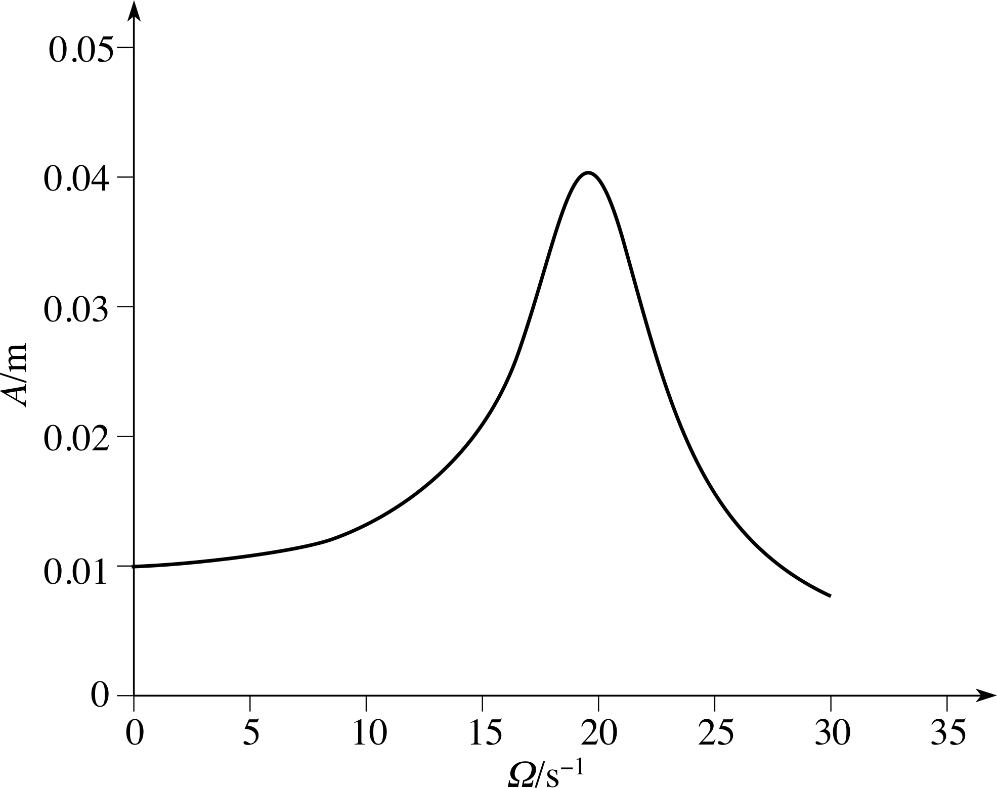
Figure 8 Graph of A as a function of Ω, in the case m = 0.2 kg, b = 1.0 N s m−1, k = 80 N m−1, F0 = 0.8 N.
that the amplitude A of the oscillations depends not only on F0, but also on Ω; in other words, applied forces of different frequency may invoke oscillations of the mass of very different magnitude.
Figure 8 shows A as a function of Ω, for a certain choice of the parameters m, k, b and F0. You can see that it has a pronounced maximum at a value of Ω close to the natural angular frequency ω0 = k.
This large response for a particular value of the angular frequency of the applied force is the well–known phenomenon of resonance. i
The above example involved some rather unpleasant algebra (because we wished to discuss a general case), however, finding the general solution to a specific inhomogeneous equation is generally straightforward enough – provided, of course, that f (t) is one of the functions mentioned in Rules 1–3 at the end of Subsection 2.6 – the method is summarized here:
- 1
-
Find the complementary function, using the methods of Subsection 2.5
- 2
-
Find the particular solution, using one of Rules 1–3 in Subsection 2.6
- 3
-
Add the two together.
You can practise these steps by trying the following question.
Question T14
Find the general solution to the equation
$\dfrac{d^2y}{dt^2} + 6\dfrac{dy}{dt} + 9y =1+3t$
Answer T14
First, we find the complementary function – the general solution to
$\dfrac{d^2y}{dt^2} + 6\dfrac{dy}{dt} + 9y = 0$
Here, a = 1, b = 6, c = 9, so b2 − 4ac = 0 and the auxiliary equation has just one root, namely −3. Thus using Equation 40,
y (t) = (B + Ct) exp[−bt/(2a)](Eqn 40)
the general solution is (B + Ct) exp(−3t).
Next, we find the particular solution. Since f (t) is a polynomial of degree 1, we try a solution of the form y = Ht + K, where H and K are undetermined coefficients. On substitution into the differential equation, we obtain
6H + 9 (Ht + K) = 1 + 3t
This is an identity, provided that the coefficients of t, and the constant terms, on each side are equal. So we have
9H = 3, 6H + 9K = 1; solving these gives us H = 1/3, K − 1/9. Thus y = t/3 − 1/9 is the particular solution.
The general solution is the sum of the complementary function and the particular solution:
y = (B + Ct) exp(−3t) + t/3 − 1/9
3 Closing items
3.1 Module summary
- 1
-
A linear differential equation with constant coefficients has the form:
$a\dfrac{d^2y}{dt^2} + b\dfrac{dy}{dx} + cy = f(t)$(Eqn 5)
If f (t) in Equation 5 is set to zero it is a linear homogeneous differential equation. If f (t) is not zero in
Equation 5 it is a linear inhomogeneous differential equation.
- 2
-
Equations of the form
$\dfrac{d^2y}{dt^2} = f(t)$(Eqn 9)
can be solved by Subsection 2.2direct integration.
- 3
-
The general solution of the SHM (simple harmonic motion) equation
$\dfrac{d^2y}{dt^2} + \omega_0^2y = 0$ (SHM equation)(Eqn 15)
can be written either as
y (t) = B cos(ω0t) + C sin(ω0t)(Eqn 16)
ory (t) = A sin(ω0t + ϕ)(Eqn 19)
corresponding to sinusoidal oscillations of period 2π/ω0. The values A and ϕ are determined from values of B and C (or vice versa) by Equations 17, 20 and 21.
B = A sin ϕ and C = A cos ϕ(Eqns 17a, b)
$A = \sqrt{B^2 + C^2}$ (positive square root)(Eqn 20)
$\dfrac BC = \dfrac{A\sin\varphi}{B\cos\varphi} = \tan\varphi$ i.e. ϕ = arctan(B/C) but with 0 ≤ ϕ < 2π(Eqn 21)
- 4
-
The Subsection 2.4general solution of an equation of the form
$\dfrac{d^2y}{dt^2} - \lambda^2 y = 0$(Eqn 23)
isy (t) = Beλt + Ce−λt(Eqn 26)
- 5
-
The nature of the solution of the (Subsection 2.5damped harmonic motion) equation
$a\dfrac{d^2y}{dt^2} + b\dfrac{dy}{dt} + cy = 0$(Eqn 29)
depends upon the sign of b2 − 4ac.
The case where b2 > 4ac corresponds to heavy damping, as illustrated in Figure 6 (with the solution given by Equation 33),
y (t) = B exp(p1t) + C exp(p2t)(Eqn 33)
where$p_1 = \dfrac{-b+\sqrt{b^2-4ac}}{2a}\quad\text{and}\quad p_2 = \dfrac{-b-\sqrt{b^2-4ac}}{2a}$
The case where b2 < 4ac corresponds to light damping, as illustrated in Figure 7 (with the solution given by Equation 37, or alternatively Equation 39),
y (t) = exp(−γt/2)[(B cos(ωt) + C sin(ωt)](Eqn 37)
y (t) = A exp(−γt/2) sin(ωt + ϕ)(Eqn 39)
The case where b2 = 4ac corresponds to critical damping (with the solution given by Equation 40),
y (t) = (B + Ct) exp[−bt/(2a)](Eqn 40)
- 6
-
To solve the (Subsection 2.5damped, driven harmonic motion) equation
$a\dfrac{d^2y}{dt^2} + b\dfrac{dy}{dt} + c = f(t)$
we first obtain the complementary function by finding a general solution of the equation
$a\dfrac{d^2y}{dt^2} + b\dfrac{dy}{dt} + c = 0$
The Subsection 2.5general solution of $a\dfrac{d^2y}{dt^2} + b\dfrac{dy}{dt} + c = f(t)$ can then be found, if we know one particular solution, by adding the complementary function to that particular solution.Particular solutionParticular solutions can be found by the method of undetermined coefficients if f (t) is a polynomial, an exponential function, or a sinusoidal function.
In the case of a sinusoidal function f (t), the amplitude of the solution (for large values of t) is dependent upon the angular frequency of f. In some cases this amplitude may be very large for a particular choice of the applied angular frequency, leading to the phenomenon of resonance.
3.2 Achievements
Having completed this module, you should be able to:
- A1
-
Define the terms that are emboldened and flagged in the margins of the module.
- A2
-
Recognize linear differential equations with constant coefficients and distinguish between homogeneous and inhomogeneous linear differential equations.
- A3$\vphantom{\dfrac{d^2}{t^2}}$
-
Solve equations of the form $\dfrac{d^2y}{dt^2} = f(t)$ by direct integration.
- A4
-
Recognize the SHM equation whenever it arises, identify the parameter ω that determines the period of oscillations and solve the equation.
- A5
-
Convert between a particular solution of the form y = B cos(ωt) + C sin(ωt) and one of the form y = A sin(ωt + ϕ) and vice versa.
- A6$\vphantom{\dfrac{d^2}{t^2}}$
-
Solve an equation of the form $\dfrac{d^2y}{dt^2} - \lambda^2 y = 0$.
- A7$\vphantom{\dfrac{d^2}{t^2}}$
-
Solve an equation of the form $a\dfrac{d^2y}{dt^2} + b\dfrac{dy}{dt} + cy = 0$, and describe the forms of the solution in the cases
b2 > 4ac, b2 < 4ac and b2 = 4ac.
- A8
-
Use the method of undetermined coefficients to find particular solutions of an equation of the form
$a\dfrac{d^2y}{dt^2} + b\dfrac{dy}{dt} + cy = f(t)$(Eqn 5)
in the cases where f (t) is a polynomial, an exponential, or a sinusoidal function.
- A9
-
Find the complementary function of an equation of the type given in Equation 5 and use it with the particular solution to obtain the general solution.
Study comment You may now wish to take the following Exit test for this module which tests these Achievements. If you prefer to study the module further before taking this test then return to the topModule contents to review some of the topics.
3.3 Exit test
Study comment Having completed this module, you should be able to answer the following questions, each of which tests one or more of the Achievements.
Question E1 (A2 and A3)
The differential equation
$\dfrac{d^2x}{dt^2} = g{\rm e}^{-kt}$
where g is the magnitude of the acceleration due to gravity and k is a positive constant, may be used to model the motion of a parachutist falling under gravity. The x–axis is chosen to be the downward vertical, with x = 0 when t = 0.
Is this equation linear, linear with constant coefficients, or homogeneous?
Find the particular solution if the parachutist starts from rest.
Answer E1
This equation is linear with constant coefficients, but it is not homogeneous.
To solve the equation, we may integrate directly. Integrating once gives us
$\dfrac{dx}{dt} = \Int g{\rm e}^{-kt}\,dt = -\dfrac gk {\rm e}^{-kt} + B$
where B is an arbitrary constant.
Since the parachutist starts from rest, dx/dt = 0 at t = 0, so that B = g/k. We now integrate again:
$x = \dfrac gk \Int(1-{\rm e}^{-kt})\,dt = \dfrac gk t + \dfrac{g}{k^2} {\rm e}^{-kt} + C$
where C is an arbitrary constant. Since x = 0 at t = 0, C = −g/k2. So the particular solution is
$x = \dfrac gk t + \dfrac{g}{k^2} \left({\rm e}^{-kt}-1\right)$
(Reread Subsection 2.1 if you had difficulty with this question.)
Question E2 (A4)
If the Earth is represented by a sphere of uniform density, the gravitational force on a particle of mass m inside the Earth at a distance r from the centre is of magnitude mgr/R, and is directed towards the centre of the Earth, where R = 6 400 km is the (approximate) radius of the Earth and g is the magnitude of the acceleration due to gravity at the Earth’s surface. If it were possible to pass a straight tube through the centre of the Earth, show that a particle placed in the tube would execute simple harmonic motion, and find the period of the motion. (Take g as 10 m s−2).
Answer E2
Applying Newton’s second law, $m\dfrac{d^2r}{dt^2} = F_r$, and putting $F_r = -\dfrac{mgr}{R}$ we find
$m\dfrac{d^2r}{dt^2} = -\dfrac{mgr}{R}$ i.e. $\dfrac{d^2r}{dt^2} + \dfrac gR r = 0$
which is the SHM equation with $\omega_0= \sqrt{gR\os}$. The period of the motion is 2π/ω0, or $2\pi\sqrt{Rg\os}$. Taking R = 6 400 km and g = 10 m s−2, this gives the value 5 030 s, or 84 min, for the period.
(Reread Subsection 2.3 if you had difficulty with this question.)
Figure 1 See Question E3.
Question E3 (A4 and A5)
The current in the circuit shown in Figure 1 satisfies the differential equation
$L\dfrac{d^2I}{dt^2} + \dfrac IC = 0$
If L = 0.02 mH, C = 3.2 × 10⁻¹⁰ F, and if I = 2.5 mA and dI/dt = −3.75 × 10⁴ A s−1 at t = 0, find the particular solution for I, both in the form B cos(ω0t) + C sin(ω0t), and in the form A sin(ω0t + ϕ).
Answer E3
Here, $\omega_0= 1/\sqrt{LC\os}$ = 1.25 × 10⁷ s−1. Writing the general solution as I = B cos(ω0t) + Csin(ω0t) we see that
dI/dt = −ω0B sin(ω0t) + ω0C cos(ω0t)
Putting t = 0, I = 2.5 mA, dI/dt = −3.75 × 10⁴ A s−1 into these equations, we find
B = 2.5 mA and −3.75 × 10⁴ A s−1 = ω0C
soC = (−3.75 × 10⁴/1.25 × 107) A = −3.0 mA
Thus
I = [2.5 cos(1.25 × 10⁷t) − 3.0 sin(1.25 × 10⁷t)] mA
where t represents the numerical value of the time in seconds.
We then use Equations 20, 21 and 22 to determine A and ϕ:
$A = \sqrt{B^2 + C^2}$ (positive square root)(Eqn 20)
$\dfrac BC = \dfrac{A\sin\varphi}{B\cos\varphi} = \tan\varphi$ i.e. ϕ = arctan(B/C) but with 0 ≤ ϕ < 2π(Eqn 21)
B ≥ 0 and C ≥ 0 ⇒ 0 ≤ ϕ ≤ π/2(Eqn 22a)
B ≥ 0 and C < 0 ⇒ π/2 < ϕ ≤ π(Eqn 22b)
B < 0 and C < 0 ⇒ π < ϕ < 3π/2(Eqn 22c)
B < 0 and C ≥ 0 ⇒ 3π/2 ≤ ϕ < 2π(Eqn 22d)
From Equation 20, $A = \sqrt{2.5^2+3.0^2}$ mA = 3.9 mA. From Equation 21, ϕ = arctan(−2.5/3.0) = 2.45 or 2.45 + π. From Equation 22, we see that since B is positive and C is negative, π/2 ≤ ϕ < π. So ϕ = 2.45. Thus
I = [3.9 sin(1.25 × 10⁷t + 2.45)] mA
(Reread Subsection 2.3 if you had difficulty with this question.)
Question E4 (A2, A4 and A6)
In a certain medium, the z–component of the electric field, Ez, varies with x, the distance from the boundary of the medium, according to the equation
$\dfrac{d^2E_z}{dx^2} + \dfrac{{\it\Omega}^2}{c^2}E_z - \mu^2E_z = 0$
where Ω, c and μ are positive constants. i Find the general solution to this equation in the three cases:
(a) Ω > μc (b) Ω = μc (c) Ω < μc
Answer E4
(a) If Ω > μc, then this equation is of the SHM type, with $\omega = \sqrt{({\it\Omega}c)^2-\mu^2}$. So the general solution is given by Equation 16,
y (t) = B cos(ω0t) + C sin(ω0t)(Eqn 16)
as $E_z = B\cos\left\{\left[\sqrt{\left({\it\Omega}c\right)^2-\mu^2}\right]x\right\} + C\sin\left\{\left[\sqrt{\left({\it\Omega}c\right)^2-\mu^2}\right]x\right\}$
(b) If Ω = μc, then d2Ez /dx2 = 0, and the equation may be integrated directly to give Ez = Bx + C.
(c) If Ω < μc, then the equation is of the type $\dfrac{d^2y}{dt^2} - \lambda^2 y = 0$, with $\lambda = \sqrt{\mu^2-\left({\it\Omega}c\right)^2}$. From Equation 26,
y (t) = Beλt + Ce−λt(Eqn 26)
the general solution is
$E_z = B\cos\left\{\left[\sqrt{\mu^2-\left({\it\Omega}c\right)^2}\right]x\right\} + C\sin\left\{\left[\sqrt{\mu^2-\left({\it\Omega}c\right)^2}\right]x\right\}$
(Reread Subsection 2.3Subsections 2.3 and Subsection 2.42.4 if you had difficulty with this question.)
Figure 5 A circuit containing an inductance L, a resistor R and a capacitor C, connected in series.
Question E5 (A7)
In the circuit shown in Figure 5, L has the value 0.02 mH and C has the value 3.2 × 10⁻¹⁰ F. The current in the circuit satisfies Equation 28,
$L\dfrac{d^2I}{dt^2} + R\dfrac{dI}{dt} + \dfrac IC = 0$(Eqn 28)
For what values of R will the current display lightly damped, oscillatory behaviour?
Find the general solution to Equation 28 if (a) R = 300 Ω, (b) R = 1300 Ω and (c) R = 500 Ω.
Answer E5
From Equation 28,
$L\dfrac{d^2I}{dt^2} + R\dfrac{dI}{dt} + \dfrac IC = 0$(Eqn 28)
we see that here a = L = 0.02 mH, b = R and c = 1/C = (3.2 × 10⁻¹⁰ F)−1 = 3.125 × 10⁹ F−1. For lightly damped behaviour, we must have b2 − 4ac < 0, or R2 < 2.5 × 10⁵ Ω2, i.e. R < 500 Ω.
(a) If R = 300 Ω, then b2 − 4ac = −1.6 × 10⁵ Ω2 < 0. We use Equation 38,
γ = b/a(Eqn 38a)
$\omega = \sqrt{4ac-b^2}/(2a)$(Eqn 38b)
to evaluate γ and ω, and find:
γ = (300) s−1/(0.02 × 10−3) = 1.5 × 10⁷ s−1
ω = (400) s−1/(2 × 0.02 × 10−3) = 1.0 × 10⁷ s−1
So from Equation 37,
y (t) = exp(−γt/2)[(B cos(ωt) + C sin(ωt)](Eqn 37)
the general solution is
I = exp(−7.5 × 10⁶t) × [B cos(1.0 × 10⁷t) + C sin(1.0 × 10⁷t)]
where t represents the numerical value of the time in seconds.
(b) If R = 1300 Ω, then b2 − 4ac = 1.44 × 10⁶ Ω2 > 0. The roots of the auxiliary equation are
p1 = −(100) s−1/(2 × 0.02 × 10−3) = −0.25 × 1071s−1
andp2 = −(2500) s−1/(2 × 0.02 × 10−3)1 = −6.25 × 10⁷ s−1
Thus from Equation 33,
y (t) = B exp(p1t) + C exp(p2t)(Eqn 33)
the general solution is
I = B exp(−0.25 × 10⁷t) + C exp(−6.25 × 10⁷t)
(c) If R = 500 Ω, then b2 − 4ac = 0, and the general solution is given by Equation 40,
y (t) = (B + Ct) exp[−bt/(2a)](Eqn 40)
With
b/2a = (500) s−1/(2 × 0.02 × 10−3) = 1.25 × 10⁷ s−1
we obtain
I = (B + Ct) exp(−1.25 × 10⁷t)
(Reread Subsection 2.5 if you had difficulty with this question.)
Question E6 (A8 and A9)
(a) Explain what is meant by the term complementary function.
(b) Find the general solution to the differential equation:
$\dfrac{d^2y}{dt^2} + \omega_0^2 y = A\cos({\it\Omega}t)$
where ω, A, Ω are constants and Ω ≠ ω0.
Answer E6
(a) The complementary function forms part of the general solution to an equation of the form
$a\dfrac{d^2y}{dt^2} + b\dfrac{dy}{dt} + cy = f(t)$
and is the general solution of the corresponding homogeneous equation
$a\dfrac{d^2y}{dt^2} + b\dfrac{dy}{dt} + cy = 0$
(b) We first find the complementary function, i.e. the solution to
$\dfrac{d^2y}{dt^2} + \omega_0^2 y = 0$
This is simply Equation 16,
y (t) = B cos(ω0t) + C sin(ω0t)(Eqn 16)
Next, we find the particular solution. Since f (t) is a sinusoidal function in this case, we try a solution of the form H cos(Ωt) + K sin(Ωt). On substitution, we obtain
−Ω2[H cos(Ωt) + K sin(Ωt)] + ω2[H cos(Ωt) + K sin(Ωt)]= Acos(Ωt)
and if this is to be an identity, the coefficients of cos(Ωt) and of sin(Ωt) on each side must be equal, giving H (ω2 − Ω2) = A and K (ω2 − Ω2) = 0. We are told that ω2 − Ω2 ≠ 0, so K = 0 and H = A/(ω2 − Ω2). Thus [A/(ω2 − Ω2)] cos(Ωt) is a particular solution.
The general solution is obtained by adding the complementary function to the particular solution; it is
$y = \dfrac{A}{\omega^2-{\it\Omega}^2}\cos({\it\Omega}t) + B\cos(\omega_0t) + C\sin(\omega_0t)$
Note that if Ω2 = ω02 our trial solution will not work – the left–hand side vanishes, whatever the values of H and K. This is because H cos(Ωt) + K sin(Ωt) is, in that case, simply the complementary function.
(Reread Subsection 2.6 if you had difficulty with this question.)
When you have completed the Exit test go back and try the Subsection 1.2Fast track questions if you have not already done so.
If you have completed both the Fast track questions and the Exit test, then you have finished the module and may leave it here.
Study comment Having seen the Fast track questions you may feel that it would be wiser to follow the normal route through the module and to proceed directly to the following Ready to study? Subsection.
Alternatively, you may still be sufficiently comfortable with the material covered by the module to proceed directly to the Section 3Closing items.