MATH 6.2: Solving first–order differential equations |
PPLATO @ | |||||
PPLATO / FLAP (Flexible Learning Approach To Physics) |
||||||
|
1 Opening items
1.1 Module introduction
First-order differential equations such as
$\dfrac{dN}{dt} = -\lambda N\quad\text{and}\quad\dfrac{dI}{dt} = -\dfrac{RC}{L}{\rm e}^{-Rt/L}$
arise in many physical contexts. The defining characteristic that is common to all such equations is that they contain no derivatives higher than the first; apart from this basic requirement they are free to take any form.
This module introduces methods that can be used to solve four different types of first–order differential equation, namely:
- 1
-
$\dfrac{dy}{dx} = f(x)$, which can be solved by direct integration;
- 2
-
$\dfrac{dy}{dx} = h(y)$, which can be solved by inversion followed by direct integration;
- 3
-
$\dfrac{dy}{dx} = f(x)h(y)$, which can be solved by separation of variables;
- 4
-
$a\dfrac{dy}{dx}+ by = f(x)$ (where a and b are constants), which can be solved by means of an integrating factor.
The discussion of these techniques occupies Subsection 2.1Subsections 2.1 to Subsection 2.42.4 of the module. The technique of changing variables, which can sometimes be usefully applied to equations that are not of any of the forms listed above is briefly considered in Subsection 2.5. Throughout the module physical examples are used to illustrate the various types of equation, but it is the mathematical aspects of the solution that are the main focus of interest.
Study comment Having read the introduction you may feel that you are already familiar with the material covered by this module and that you do not need to study it. If so, try the following Fast track questions. If not, proceed directly to the Subsection 1.3Ready to study? Subsection.
1.2 Fast track questions
Study comment Can you answer the following Fast track questions? If you answer the questions successfully you need only glance through the module before looking at the Subsection 3.1Module summary and the Subsection 3.2Achievements. If you are sure that you can meet each of these achievements, try the Subsection 3.3Exit test. If you have difficulty with only one or two of the questions you should follow the guidance given in the answers and read the relevant parts of the module. However, if you have difficulty with more than two of the Exit questions you are strongly advised to study the whole module.
Question F1
Find the general solution of the following differential equations:
(a) $\dfrac{dy}{dx} = \dfrac{x}{\sqrt{4-x^2}}$ (where −2 < x < 2)
(b) $2x^{1/2}y\dfrac{dy}{dx} = 1$ (where x > 0)
(c) $\dfrac{dy}{dx} = 1 - y^2$ (where −1 < y < 1)
Answer F1
(a) This differential equation can be solved by direct integration:
$\displaystyle y = \int{x}{\sqrt{4-x^2}} = -\sqrt{4-x^2} + C$, where C is a constant of integration.
Notice that the condition −2 < x < 2 ensures that the first expression on the right–hand side of this equation is
real.
(b) This equation can be solved by separation of variables, to give
$2\Int y\,dy = {\displaystyle \int}\dfrac{1}{x^{1/2}}$, or y = 2x1/2 + C, where C is a constant of integration.
Making y the subject, we obtain $y = \pm\sqrt{2x^{1/2} + C}$ (the condition x > 0 ensures that x1/2 is real).
(c) This equation is solved by first using the inversion rule, to obtain
$\dfrac{dx}{dy} = \dfrac{1}{1-y^2}$, which can be directly integrated to give
$\displaystyle x = \int\dfrac{1}{1-y^2}\,dy$
To evaluate this integral, use partial fractions to write
$\dfrac{1}{1-y^2} = \dfrac{1}{2(1+y)} + \dfrac{1}{2(1-y)}$
so that
${\displaystyle x = \int\dfrac{1}{2(1+y)}\,dy + \int\dfrac{1}{2(1-y)}\,dy} = \frac12 \loge(1+y)-\frac12\loge(1-y) + C$
where C is a constant of integration.
Exponentiating both sides and performing a little manipulation gives us:
$\dfrac{1+y}{1-y} = C_1{\rm e}^{2x}$
where C1 = e−2C is another arbitrary constant.
Finally, making y the subject gives us $y = \dfrac{C_1{\rm e}^{2x}-1}{C_1{\rm e}^{2x}+1}$
Question F2
Explain what is meant by an integrating factor. Use the method of integrating factors to find the general solution of the differential equation
$2\dfrac{dy}{dx} = x-4y$
and find the particular solution if y = 1/2 at x = 0.
Answer F2
An integrating factor is a function by which each term of a linear first–order differential equation is multiplied to enable integration to be performed.
This differential equation is a linear equation with constant coefficients and can be written in the form
$\dfrac{dy}{dx} + 2y = \dfrac x2$
The integrating factor for such an equation is exp(2x). Multiplying the equation by exp(2x) gives
$\dfrac{d}{dx}\left(y{\rm e}^{2x}\right) = \dfrac x2 {\rm e}^{2x}$
which can be directly integrated, to give $\displaystyle y{\rm e}^{2x} = \int \dfrac x2 {\rm e}^{2x}\,dx$
The integral can be evaluated using integration by parts to give $y{\rm e}^{2x} = \frac14 x{\rm e}^{2x} - \frac 18 {\rm e}^{2x}+ C$, where C is a constant of integration.
So$y =\frac14x - \frac18 + C{\rm e}^{-2x}$ is the general solution. Substituting $y = \frac12$ at x = 0, we find $C = \frac58$; thus the particular solution is $y = \frac14x -\frac18 + \frac58{\rm e}^{-2x}$.
Study comment Having seen the Fast track questions you may feel that it would be wiser to follow the normal route through the module and to proceed directly to the following Subsection 1.3Ready to study? Subsection. Alternatively, you may still be sufficiently comfortable with the material covered by the module to proceed directly to the Section 4Closing items.
1.3 Ready to study?
Study comment In order to study this module you will need to understand the following terms: constant of integration, dependent variable, derivative, general solution, independent variable, initial condition, inverse derivative (i.e. indefinite integral), linear differential equation and particular solution. You will need to have a good knowledge of differentiation (including the product_rule_of_differentiationproduct and chain_rulechain rules, and implicit differentiation), and of integration methods (including integration by substitution, integration by parts and the use of partial fractions); you should be familiar with the idea of checking a solution_mathematicalsolution to a differential equation by substitution. If you are uncertain about any of these terms, you can review them by reference to the Glossary, which will also indicate where in FLAP they are developed. You should note that throughout this module $\sqrt{x\os}$ represents the positive square root of x. The following questions will allow you to establish whether you need to review some of these topics before embarking on this module.
Question R1
Use the product_rule_of_differentiationproduct and chain_rulechain rules to express the derivative
$\dfrac{d}{dx}(x^3\loge y)$
in terms of x, y and dy/dx. (This kind of differentiation is known as implicit differentiation.)
Answer R1
We use the product_rule_of_differentiationproduct rule to differentiate the product, and the technique of implicit differentiation to differentiate loge y. This gives
$\dfrac{d}{dx}\left(x^3\loge y\right) = x^3\dfrac{d}{dx}\left(\loge y\right) + 3x^2\loge y = \dfrac{x^3}{y}\dfrac{dy}{dx} + 3x^2\loge y$
(If you are uncertain about these terms consult the Glossary.)
Question R2
Determine the inverse derivatives (i.e. the indefinite integrals) of the following functions of x:
(a) x e−x (b) ex cos x
Answer R2
These indefinite integrals can both be evaluated using integration by parts. (In the following answers C stands for a constant of integration.)
(a) $\Int x{\rm e}^{-x}\,dx = -x{\rm e}^{-x} + \Int{\rm e}^{-x}\,dx = -(x+1){\rm e}^{-x} + C$
(b) ${\rm e}^x\cos x\,dx = {\rm e}^x\sin x - {\rm e}^x\sin x\,dx = {\rm e}^x\sin x + e{\rm e}^x\cos x- {\rm e}^x\cos x\,dx$
So$2\Int {\rm e}^x\cos x\,dx = {\rm e}^x\sin x + {\rm e}^x\cos x$
i.e.$\Int {\rm e}^x\cos x\,dx = \frac12{\rm e}^x(\sin x + \cos x) + C$
(If you are uncertain about these terms consult the Glossary.)
Question R3
By making suitable substitutions, evaluate the following indefinite integrals:
(a) $\displaystyle \int x\exp\left(\dfrac{x^2}{2}\right)\,dx$ (b) $\Int\sin x(\cos x)^6\,dx$ (c) $\Int\sqrt{1-x\os}\,dx$
Answer R3
These integrals can all be evaluated by means of an appropriate substitution.
(a) To evaluate $\Int x\exp\left(\dfrac{x^2}{2}\right)\,dx$, use the substitution u = x2/2 so du = xdx. The integral becomes
$\Int {\rm e}^u\,du = {\rm e}^u + C = {\rm e}^{x^2/2} + C$
(b) To evaluate $\Int\sin x(\cos x)^6\,dx$ use the substitution u = cos x so du = −sin x dx. The integral becomes
$-\Int u^6\,du = -u^7/7 + C = -(\cos x)^7/7 + C$
(c) To evaluate $\Int\sqrt{1-x\os}\,dx$ use the substitution u = 1 − x, so du = −dx. The integral becomes
$-\Int\sqrt{u\os}\,du = -\dfrac23u^{3/2} + C = -\dfrac23(1-x)^{3/2} + C$
(If you are uncertain about these terms consult the Glossary.)
Question R4
By using partial fractions, evaluate $\displaystyle \int \dfrac{1}{x(x+3)}\,dx$
Answer R4
To evaluate this integral, first use the technique of partial fractions, to write the integrand as $\dfrac{1}{3x} - \dfrac{1}{3(x + 3)}$
Integrating both these terms then gives the result
$\displaystyle \int \dfrac{1}{x(x+3)}\,dx = \dfrac13\loge x - \dfrac13\loge(x+3) + C = \dfrac13\loge\left(\dfrac{x}{x+3}\right) + C$
(If you are uncertain about these terms consult the Glossary.)
Question R5
Explain the difference between a general solution and a particular solution of a first–order differential equation.
Answer R5
A general solution to a first–order differential equation is a solution that contains one arbitrary constant. A particular solution contains no arbitrary constant. (If you are uncertain about these terms consult the Glossary.)
Question R6
Show by substitution that
$I = \dfrac ER + C{\rm e}^{-Rt/L}$
where C is an arbitrary constant, is a solution_mathematicalsolution of the differential equation
$L\dfrac{dI}{dt} + RI = E$ where L, R and E are given constants.
Find the value of the arbitrary constant C in terms of E and R, given I = 0 at t = 0.
Answer R6
Differentiating $I = \dfrac ER + C{\rm e}^{-Rt/L}$ with respect to t gives us
$\dfrac{dI}{dt} = -\dfrac{RC}{L}{\rm e}^{-Rt/L}$
and substituting this, and the expression for I, into the left–hand side of the differential equation gives us
$L\dfrac{dI}{dt} + RI = -RC{\rm e}^{-Rt/L} + E + RC{\rm e}^{-Rt/L}$
which is identically equal to E. So the differential equation is satisfied. Substituting t = 0 and I = 0 into the solution, we find C = −E/R.
(If you are uncertain about these terms consult the Glossary.)
Comment Many of the Text questions that follow involve the evaluation of an indefinite integral as one of the steps. In the solutions, a detailed explanation of how the integral is to be evaluated is not given. If you have trouble with any of these integrals, you should consult the Glossary, or one of the modules dealing with integration.
2 Methods of solution for various first–order differential equations
Notation When a general type of differential equation is discussed in this module the independent variable will be denoted by x and the dependent variable by y. However, many of the examples given in this module are drawn from problems in physics, where the context suggests more appropriate symbols for the independent and dependent variables. Other examples involve purely ‘abstract’ differential equations and may also use a different notation. Bear in mind that the quantity being differentiated will always be the dependent variable.
For each of the four methods described in Subsection 2.1Subsections 2.1 to Subsection 2.42.4, a particular example from physics is used as an illustration.
2.1 Equations of the form dy/dx = f (x); direct integration
There is a whole class of first–order differential equations that you can already solve. In general, these equations are of the form:
$\dfrac{dy}{dx} = f(x)$(1)
where the derivative of the dependent variable is equal to a given function of the independent variable. A typical example of this type of differential equation is dy/dx = cos x. If the derivative of y is equal to f (x), then, by definition, y is the inverse derivative of f (x), or, in other words, the indefinite integral of f (x). Thus the solution to Equation 1 can be written simply as an integral:
$y = \Int f(x)\,dx$(2)
In the particular case dy/dx = cos x we have f (x) = cos x and therefore
$y = \Int\cos x\,dx = \sin x + C$ (where C is an arbitrary constant i).
In general, when we evaluate the indefinite integral in Equation 2, we will introduce an arbitrary constant of integration; hence Equation 2 gives us the general solution of Equation 1.
The following differential equation can be solved by this method, which is known as the method of direct integration:
Example 1
Find the general solution of the differential equation
$\dfrac{dy}{dx} = {\rm e}^{2x}\,dx$
Solution
The general solution is
$y = \Int{\rm e}^{2x}\,dx$
that is $y = \frac12{\rm e}^{2x} + C$(3)
Question T1
Can the direct integration method be applied to the following differential equations? Find the general solution of the equation in those cases where the method can be applied.
(a) $\dfrac{dy}{dx} = x\sin x$ (b) $\dfrac{dy}{dx} = y\sin y$
Answer T1
(a) Direct integration can be used here, as the right–hand side is only a function of x, the independent variable. The general solution is $y = \Int x\sin x\,dx$, which can be evaluated using integration by parts, to give
y = −x cos x + sin x + C
(b) Here, x is the dependent variable. Thus the right–hand side is a function of the dependent variable, so direct
integration cannot be used.
Very often the solution of such a problem in physics requires a particular rather than a general solution, which means that we need an extra piece of information in order to assign an appropriate value to the arbitrary constant. This extra piece of information is often provided in the form of an initial condition. For example, suppose that in Example 1 we are told that y = 2 when x = 0. Substituting these values into Equation 3, we obtain $2 = \dfrac{{\rm e}^0}{2} + C$, i.e. C = 3/2. Thus the particular solution, satisfying both the differential equation and the initial condition, is $y = \dfrac{{\rm e}^{2x}}{2} + \dfrac32$.
Resisted motion under gravity
Problems involving the motion of objects often give rise to differential equations that can be solved by direct integration, and in such cases the initial condition arises in a very natural fashion. For example, we might know the velocity vx(t) of an object as a function of time t, and want to calculate its position coordinate x as a function of time. i Since vx = dx/dt, this immediately presents us with a first–order differential equation, the general solution of which can be found simply by integrating vx with respect to t. If we are given a value of x at some particular time t, this will allow us to assign a specific value to the general solution’s arbitrary constant, and thus solve the problem completely. The following question is an example of this sort of problem.
Question T2
At time t = 0 a stone of mass m is thrown vertically upwards with initial velocity ux i (in this case we take the vertically upwards direction to be the direction of increasing x values). The upward motion of the stone is opposed by the (downward) force of gravity, −mg, and by a air_resistanceresistive force −mkvx (where k is a positive constant). The height x of the stone above its point of projection at time t (> 0) can be shown to be given by the solution of the differential equation
$\dfrac{dx}{dt} = \left(u_x + \dfrac gk\right){\rm e}^{-kt} - \dfrac gk$
(a) Find the general solution of the differential equation.
(b) Use the initial condition x = 0 at t = 0 to find an expression for the height x of the stone at time t.
Answer T2
(a) The general solution is
$\displaystyle x = \int\left[\left(u_x + \dfrac gk\right){\rm e}^{-kt}\right]\,dt$
that is, $x = -\dfrac 1k\left(u_x + \dfrac gk\right){\rm e}^{-kt} - \dfrac gk t + C$
(b) If the initial conditins t = 0 and x = 0 are substituted into the general solution, we find
$0 = -\dfrac 1k\left(u_x + \dfrac gk\right) + C$
Thus the height x of the stone at time t is
$x = -\dfrac 1k\left(u_x + \dfrac gk\right)(1 - {\rm e}^{-kt}) - \dfrac gk t$
2.2 Equations of the form dy/dx = h (y); inversion and direct integration
Another common sort of differential equation is one where the derivative is a function of the dependent variable
only; such equations have the general form:
$\dfrac{dy}{dx} = h(y)$(4)
The differential equation dy/dx = y3 is a typical example of this type of equation. Such equations can be converted into a more convenient form using a relationship called the inversion rule:
$\dfrac{dx}{dy} = \dfrac{1}{dy/dx}$(5)
A mathematical aside Since you may not be familiar with Equation 5, we will give a quick proof of it.
Suppose that y is some function of x so
y = f (x)(6)
Differentiating both sides with respect to y, we obtain
1 = df /dy(7)
To express df /dy in an alternative way, think of f as a function of a function: f is a function of x, but Equation 6 defines x as the inverse function f−1(y). So, using the chain rule we obtain
$\dfrac{df}{dy} = \dfrac{df}{dx} \times \dfrac{dx}{dy}$
but df /dx is just the same as dy/dx, so Equation 7 gives us
$1 = \dfrac{dy}{dx} \times \dfrac{dx}{dy}$, i.e. $\dfrac{dx}{dy} = \dfrac{1}{dy/dx}$
as claimed in Equation 5.
An example should make the matter clear. If y = x2 then we may differentiate with respect to x and obtain dy/dx = 2x. On the other hand, if y = x2 then $x = \sqrt{y\os} = y^{1/2}$ and therefore $\dfrac{dx}{dy} = \dfrac{y^{-1/2}}{2} = \dfrac{1}{2\sqrt{y\os}} = \dfrac{1}{2x}$, and therefore we have $\dfrac{dx}{dy} = \dfrac{1}{dy/dx}$. The following question reinforces this idea.
Question T3
Calculate dy/dx and dx/dy, and show that they satisfy the inversion rule, in each of the following cases:
(a) y = x3 (which has x = y1/3 as its inverse function)
(b) y = ex (which has x = loge y as its inverse function).
Answer T3
(a) If y = x2, dy/dx = 3x2; and from x = y2, $dx/dy =\frac13y^{-2/3} = 1/(3x^2)$.
So the product dy/dx × dx/dy is equal to 1, in agreement with the inversion rule.
(b) If y = ex, dy/dx = ex; and from x = loge y, dx/dy = 1/y = 1/ex. So the product dy/dx × dx/dy is equal to 1, in agreement with the inversion rule.
Returning to Equation 4,
$\dfrac{dy}{dx} = h(y)$(Eqn 4)
this can be rewritten, using the inversion rule, as
$\dfrac{dx}{dy} = \dfrac{1}{h(y)}$(8)
which is now in the right form to be solved by direct integration; so we have
$\displaystyle x = \int\dfrac{1}{h(y)}\,dy$
Provided that we can evaluate this indefinite integral, we can obtain x as a function of y. Ideally we should like to represent y explicitly as a function of x but this may not always be possible, and we may have to be satisfied with an equation that determines y as an implicit function of x.
✦ Find the general solution of the differential equation
$\dfrac{dy}{dx} = \dfrac{1}{5y^4+1}$
✧ If we rearrange this equation, we have
$\dfrac{dx}{dy} = 5y^4 + 1$
so that
$x = \Int(5y^4+1)\,dy = y^5+y+C$
and therefore the general solution of the differential equation is given by the implicit function y5 + y + C = x. In this case there is no explicit formula for y as a function of x.
The radioactive decay equation
As a further example of this method, let us solve Equation 9, the equation of radioactive decay
$\dfrac{dN}{dt} = -\lambda N$(9)
where N is the number of radioactive nuclei present at time t and λ is a constant characteristic of the decaying substance and is known as the decay constant.
Inversion of Equation 9 gives us
$\dfrac{dt}{dN} = - \dfrac{1}{\lambda N}$
and direct integration gives
$\displaystyle t = -\int\dfrac{1}{\lambda N}\,dN = -\lambda \int\dfrac1N\,dN = -\dfrac1\lambda\loge N + C$
so that the general solution of the differential equation is $t + \dfrac1\lambda\loge N = C$. However, it may be possible to write this equation in a neater form, so let us try to make the dependent variable, N, the subject of the equation.
If we rearrange the general solution we find
$C - t = \dfrac{1}{\lambda}\loge N$, i.e. $\loge N = \lambda(C - t)$
Using the fact that loge and exp are inverse functions, we can exponentiate both sides, to obtain
exp(loge N) = exp(λC − λt) so that N = eλC e−λt
This is a perfectly valid form of the general solution to Equation 9, but it is convenient and conventional to write it in a slightly different way. Since λ is a given constant and C is an arbitrary constant, exp(λC) is just another arbitrary constant, which we can call A. The general solution to Equation 9 can therefore be written as
N = A e−λt(10)
Having found a general solution to a differential equation, it is always a good idea to check that it is indeed a solution, by substituting it back into the original equation.
✦ Check that Equation 10 is a general solution to Equation 9.
✧ If we differentiate N = A e−λt with respect to t we get dN/dt = −λA e−λt which is equal to −λN.
So Equation 9,
$\dfrac{dN}{dt} = -\lambda N$(Eqn 9)
is satisfied.
You may find it useful to think of the technique of inversion and direct integration in four steps:
Inversion and direct integration
- 1
-
Invert $\dfrac{dy}{dx} = h(y)$ to obtain $\dfrac{dx}{dy} = \dfrac{1}{h(y)}$.
- 2
-
Integrate to obtain $\displaystyle x = \int\dfrac{1}{h(y)}\,dy$.
- 3
-
Manipulate this equation to make the dependent variable y the subject.
- 4
-
Check your general solution by substitution.
There may often be one further step – the use of an initial condition to obtain a value for the arbitrary constant appearing in the general solution. You can practise these various steps by answering the following question.
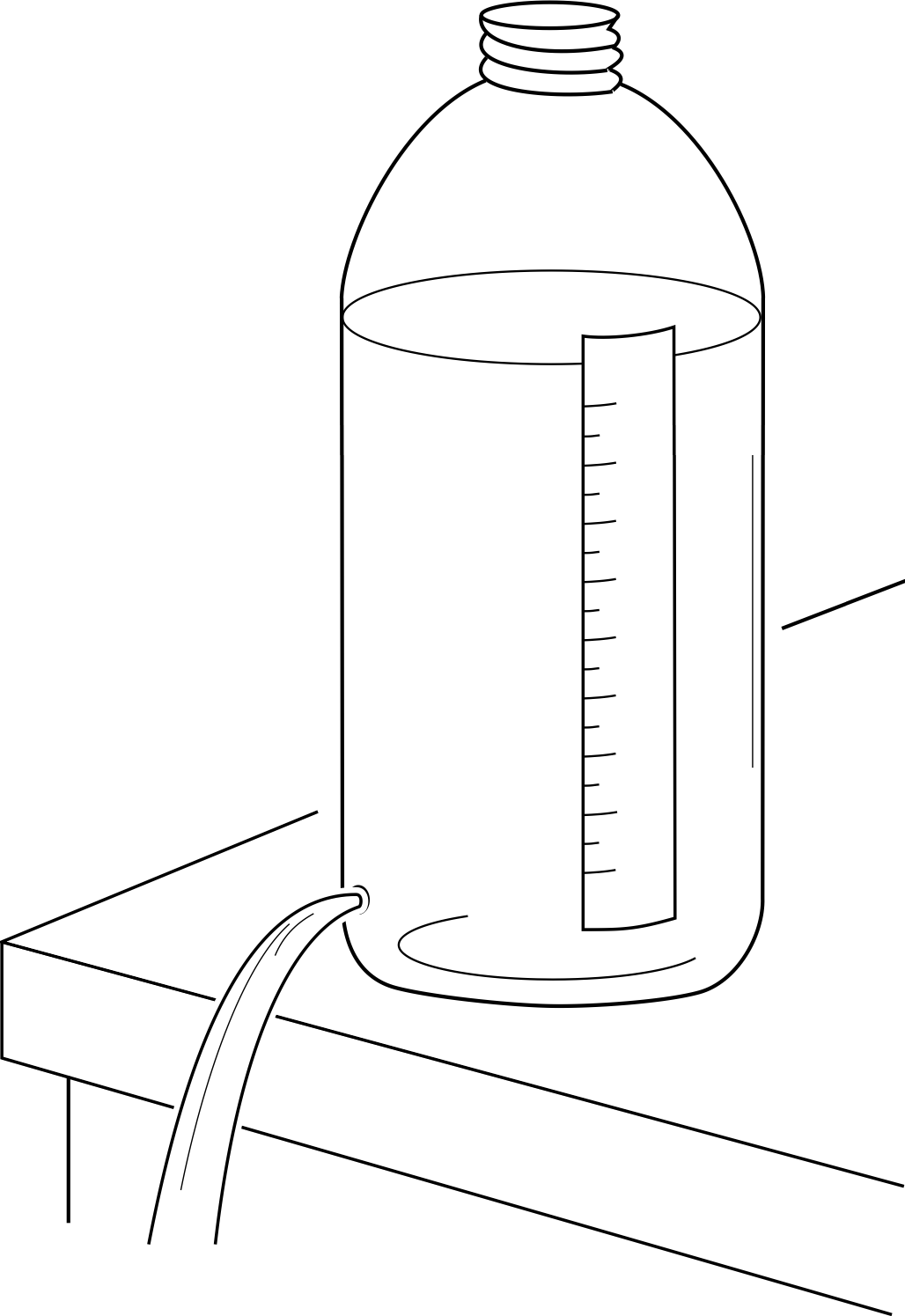
Figure 1 See Question T4.
Question T4
When water flows out of a hole in a bottle of constant cross–sectional area (see Figure 1), the height y of the water above the hole varies with time t according to the differential equation
$\dfrac{dy}{dt} = -k\sqrt{y\os}$
where k is a positive constant.
Find:
(a) the general solution of this differential equation, and
(b) the particular solution corresponding to the initial condition
y = y0 (where y0 > 0) at t = 0.
Answer T4
(a) Step 1 Inverting this differential equation gives us
$\dfrac{dt}{dy} = -\dfrac{1}{k\sqrt{y\os}}$
Step 2 Integrating gives us t as a function of y:
$\displaystyle t = -\int\dfrac{1}{k\sqrt{y\os}}\,dy = -\dfrac{2\sqrt{y\os}}{k} + C$
Step 3 Manipulating this equation to make y the subject gives the general solution $y = \frac14k^2(C-t)^2$.
Comment In these answers, we will not carry out the step of checking the solution by substitution - but you should always do so.
(b) To find the particular solution, we evaluate C by substituting y = y0 at t = 0, to obtain $y_0 = \frac14k^2C^2$, or $C = 2\sqrt{y_0\os}/k$. Thus the particular solution can be written as $y = \left(\sqrt{y_0\os} - \dfrac{kt}{2}\right)^2$.
We have now seen how to solve a first–order differential equation if the derivative of y is equal either to a function of x alone, or to a function of y alone.
In the next two subsections, we will consider some cases where the derivative is equal to a function of both x and y.
2.3 Equations of the form dy/dx = f (x)h (y); separation of variables
To illustrate the mathematics discussed here we will begin this subsection by presenting you with three differential equations, drawn from completely different branches of physics, and will then show you that they are all of the same type. After explaining the general method of solving such differential equations, we will apply the method to two of these equations, and leave you to solve the third.
Volume and pressure in a gas
The first example concerns the way in which the pressure P of a gas varies with its volume V if the gas is compressed or expanded in such a way that, though the temperature may change, no heat is allowed to enter or leave the gas. i The differential equation determining P as a function of V is
$\dfrac{dP}{dV} = -\gamma \dfrac PV$(11)
where γ is a positive constant that depends on the nature of the gas.
A space probe
For the second example, consider the case of a space probe launched vertically upwards from the Earth’s surface. When the probe is at a distance r from the centre of the Earth, its outward velocity vr satisfies the differential equation
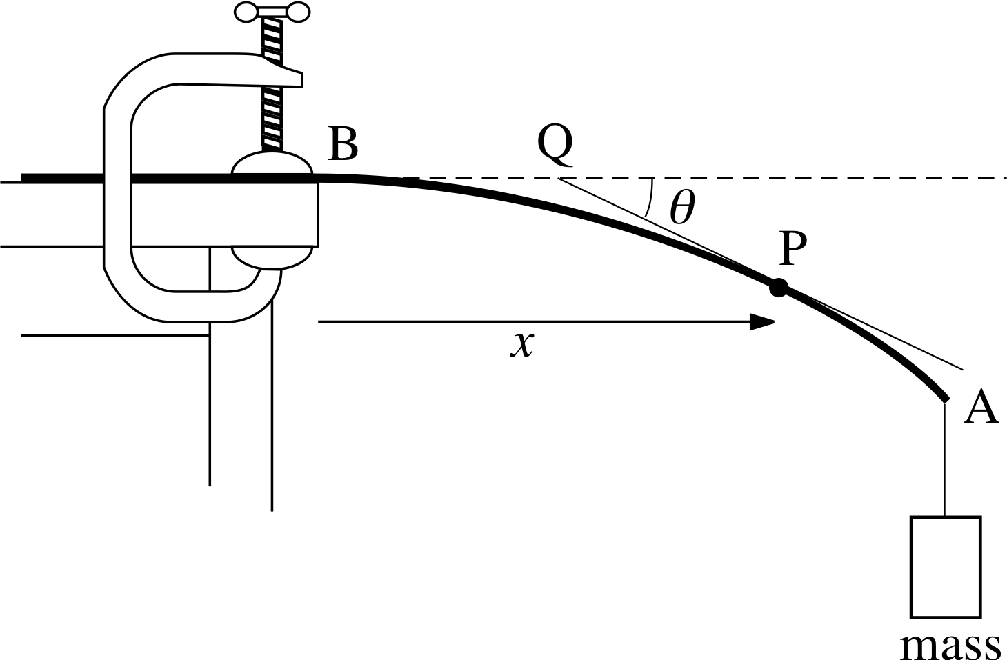
Figure 2 A flexible beam clamped at end B with a mass suspended at end A. The line PQ is a tangent to the beam at point P.
$\dfrac{dv_r}{dr} = -\dfrac{\mu}{v_r r^2}$ (for r > R and vr > 0)(12)
where R is the radius of the Earth and μ is a positive constant.
A flexible beam
Finally, Equation 13 describes the shape taken up by a thin flexible beam of length a which is caused to bend when a mass is suspended at one end, while it is clamped at the other end (see Figure 2):
$\cos\theta\dfrac{d\theta}{dx} = k(a-x)$(13)
where the variables x and θ are defined in Figure 2, and k is a positive constant.
| derivative | function of dependent variable |
function of independent variable |
|||
|---|---|---|---|---|---|
| gas | $\dfrac{dP}{dV}$ | = | P | × | $-\dfrac{\gamma}{V}$ |
| space probe | $\dfrac{dv_r}{dr}$ | = | $-\dfrac{\mu}{v_r}$ | × | $\dfrac{1}{r^2}$ |
| flexible beam | $\dfrac{d\theta}{dx}$ | = | $\dfrac{1}{\cos\theta}$ | × | k (a − x) |
Equations 11 to 13 have a common property: they may all be written in such a way that the derivative is equal to a function of the independent variable multiplied by a function of the dependent variable. Equations 11 and 12 are already in this form, but Equation 13 requires a little rewriting to make it of this type; if we divide both sides by cos θ, we obtain
$\dfrac{d\theta}{dx} = \dfrac{k(a-x)}{\cos\theta}$
Table 1 clarifies this common structure.
All these differential equations are, therefore, examples of the general form
$\dfrac{dy}{dx} = f(x)h(y)$(14)
A differential equation of this type is said to be separable, because it can be solved by a method known as separation of variables, which we will now explain.
We first rewrite Equation 14 so that there is only a function of x on the right–hand side, by dividing both sides by h (y):
$\dfrac{1}{h(y)}\dfrac{dy}{dx} = f(x)$(15a)
or$j(y)\dfrac{dy}{dx} = f(x)$(15b)
where, purely for convenience, we have introduced the notation j (y) = 1/h (y). We now integrate both sides of Equation 15b with respect to x
${\displaystyle \int} j(y)\dfrac{dy}{dx}\,dx = \Int f(x)\,dx$(16)
The right–hand side is no problem, but the left–hand side appears less straightforward. However, you should be familiar with the method of integration by substitution, which is based on a rule of the following form
$\Int j(y)\,dy = {\displaystyle \int}j(y(x))\dfrac{dy}{dx}\,dx$(17) i
the implication of this is that the expression $\left(\dfrac{dy}{dx}\right)dx$ inside the integral can be replaced by dy.
Using this result in Equation 16 gives
$\Int j(y)\,dy = \Int f(x)\,dx$
or, in terms of the function h (y),
${\displaystyle \int}\dfrac{1}{h(y)}\,dy = \Int f(x)\,dx$(18)
Provided that both integrals can be evaluated, Equation 18 gives a relation between y and x, which represents the general solution of the differential equation. This relation can sometimes be manipulated to make y its subject.
The following example should make the method of separation of variables clearer.
Example 2
Find the general solution of Equation 11,
$\dfrac{dP}{dV} = -\gamma\dfrac PV$(Eqn 11)
and express P as an explicit function of V.
Solution
If we divide by P and integrate both sides of the equation with respect to V we get
$\displaystyle \dfrac 1P\dfrac{dP}{dV}\,dV = -\gamma \int\dfrac1V\,dV$(19)
The integral on the right–hand side is simply −γ loge V + C. i To evaluate the integral on the left–hand side, use Equation 17 to write Equation 19 as
$\displaystyle \int\dfrac 1P\,dP = -\gamma\loge V + C$
which implies loge P = −γ loge V + C(20) i
Equation 20 is the general solution, but it may be possible to write it in a neater form. To do so, first make use of the fact that a function of an arbitrary constant is itself an arbitrary constant, so it is certainly possible to define a new arbitrary constant C1 by means of the equation C = loge C1. Using this new constant Equation 20 becomes
loge P = −γ loge V + loge C1 = loge(C1V−γ) exponentiating both sides then gives,
P = C1V−γ where C1 is a constant
✦ Check this general solution by substitution.
✧ If P = C1V−γ, then
$\dfrac{dP}{dV} = -\gamma C_1V^{(-\gamma+1)} = -\gamma C_1V ^{-\gamma}\times\dfrac1V = -\gamma \dfrac PV$
and so Equation 11,
$\dfrac{dP}{dV} = -\gamma\dfrac PV$(Eqn 11)
is satisfied.
A short cut There is a short cut which many people take when using the technique of separation of variables. It involves treating dy/dx as though it were ‘dy’ divided by ‘dx’. We will now show you how it works.
Earlier, we went from the differential equation
$\dfrac{1}{h(y)}\dfrac{dy}{dx} = f(x)$(Eqn 15a)
to the equation
${\displaystyle \int}\dfrac{1}{h(y)}\,dy = \Int f(x)\,dx$(Eqn 18)
by using an argument based on the rule for evaluating integrals by substitution. However, many people would bypass this rigorous argument, and instead simply ‘multiply’ both sides of Equation 15b by ‘dx’ to get
$\dfrac{1}{h(y)}\,dy = f(x)\,dx$(21)
i.e. they would ‘separate’ the ‘dy’ and ‘dx’ as well. They would then integrate both sides of this equation, and so arrive at Equation 18. There is nothing wrong with setting out your solution in this way provided you understand that it is nothing more than a notational short cut and that you appreciate the rigorous derivation (given in Equations 15–18).
Example 3
Find the general solution to Equation 12,
$\dfrac{dv_r}{dr} = -\dfrac{\mu}{v_r r^2}$ (for r > R and vr > 0)(Eqn 12)
Solution
To separate variables, multiply both sides of this equation by vr and by ‘dr’. This gives
vrdvr = −μdr/r2
(the analogue of Equation 21).
Now integrate both sides, to obtain
$\Int v_r\,dv_r = -\mu{\displaystyle \int}\dfrac{1}{r^2}\,dr$
Evaluating these integrals gives us the general solution
$\frac12 v_r^2 = \mu/r + C$
(Note that the two constants of integration have again been absorbed into one constant.)
Rearranging this equation to make vr the subject, we find
$v_r = \pm \sqrt{2(\mu/r+C)\os}$
which is the general solution of the given differential equation.
(The two possible signs for vr appear because the space probe could be moving towards or away from the Earth. As vr was defined as the outward velocity, the plus sign applies when the space probe is moving away and the minus sign when it is moving towards the Earth.)
Before you start to apply the method of separation of variables yourself, you may find a summary of the method as a series of steps helpful:
Separation of variables
- 1
-
If the differential equation is not obviously in the form
$\dfrac{dy}{dx} = f(x)h(y)$(Eqn 14)
try to write it in this form by appropriate multiplication, division or factorization. (If this cannot be done, then you must use some other method to solve the equation!)
- 2
-
Rewrite this in the form
$\dfrac{1}{h(y)}\dfrac{dy}{dx} = f(x)$(Eqn 15a)
- 3
-
Integrate both sides with respect to x to get
${\displaystyle \int}\dfrac{1}{h(y)}\,dy = \Int f(x)\,dx$(Eqn 18)
- 4
-
Evaluate the integrals, not forgetting a constant of integration.
- 5
-
If possible, manipulate the resulting equation to make y the subject.
- 6
-
Check your answer is a general solution by substitution.
You can now test your understanding of the method by answering the following two questions.
Question T5
Are the following differential equations separable?
(a) $\dfrac{dy}{dx} = x^2y^3+ x^2$ (b) $yx\dfrac{dy}{dx} = 3$ (c) $\dfrac{dy}{dx} = 2y + x^2$ (d) $\dfrac{dQ}{dt} = 2Q$
Answer T5
These equations are separable, except for (c). Note that equation (a) can be written as dy/dx = x2(1 + y3), and that in equation (d), the function of the independent variable t on the right–hand side is simply equal to 1.
Question T6
Find the general solution of Equation 13,
$\cos\theta\dfrac{d\theta}{dx} = k(a-x)$(Eqn 13)
and the particular solution corresponding to the initial condition θ = 0 at x = 0.
Answer T6
There is no need for Step 1 – it has already been explained in the text that this equation is separable.
Step 2 Separating the variables gives
$\Int\cos\theta\,d\theta = k\Int(a-x)\,dx$
Step 3 Evaluating these integrals gives
$\sin\theta = k(ax - \frac12x^2) + C$
Step 4 Making the dependent variable θ the subject gives the general solution
$\theta = \arcsin[k(ax - \frac12x^2) + C]$
Substituting θ = 0 at x = 0 gives C = 0, so the particular solution is
$\theta = \arcsin[k(ax - \frac12x^2)]$
It may have occurred to you that the two types of equation discussed in Subsection 2.1Subsections 2.1 and Subsection 2.22.2, namely,
$\dfrac{dy}{dx} = f(x)$(Eqn 1)
and$\dfrac{dy}{dx} = h(y)$(Eqn 4)
are special cases of Equation 14:
$\dfrac{dy}{dx} = f(x)h(y)$(Eqn 14)
in Equation 1, h (y) = 1; and in Equation 4, f (x) = 1. Both equations could be solved by separation of variables (compare part (d) of Question T5), but this method of solution might take rather longer than direct integration or inversion.
In each of the methods that we have discussed we are, at some stage, required to evaluate integrals, and therefore the success of the methods naturally depends on the corresponding functions being integrable. Later you may meet integrals that cannot be expressed in terms of simple functions, in which case you may need to use a numerical method, however such methods are beyond the scope of this module.
A further problem, of which you should be aware, arises from the fact that division by zero is not defined. Thus for the differential equation
$\dfrac{dy}{dx} = f(x)h(y)$
the manipulation that gives
${\displaystyle \int}\dfrac{1}{h(y)}\,dy = \Int f(x)\,dx$
is only satisfactory if h (y) ≠ 0. In Example 3 the conditions r > R and vr > 0 are sufficient to ensure that our solution is valid.
2.4 Equations of the form a (dy/dx) + by = f (x); integrating factors
You have now seen three types of first–order differential equations for which a general solution can always be found (provided, of course, that the integrals appearing in the solution can be evaluated). There is one other type of equation which (with the same proviso) can always be solved.
This is the first–order_differential_equationfirst–order linear differential equation, which has the general form
$a(x)\dfrac{dy}{dx} + b(x)y = f(x)$(22)
where a (x), b (x) and f (x) are arbitrary functions of x.
Many of the linear first–order differential equations that you are likely to meet in physics are in fact rather simpler than Equation 22, in that y and dy/dx are multiplied simply by constants instead of functions of x (though a function of x may still appear on the right–hand side). In this module we restrict our discussion to differential equations of this form.
A linear equation of this sort is called a first–order linear differential equation with constant coefficients. A first–order linear equation with constant coefficients is, therefore, of the form
$a\dfrac{dy}{dx} + by = f(x)$(23)
where a and b are constants. In this subsection we will explain how to solve differential equations of this type. First, we will look at two examples of linear first–order differential equations with constant coefficients that arise in physics. The first is a generalization of Equation 9,
$\dfrac{dN}{dt} = -\lambda N$(Eqn 9)
Radioactive decay
If a radioactive substance A is not only decaying, but is also being formed by the decay of some other radioactive substance B, then the number N of nuclei of substance A present at time t is given by the differential equation
$\dfrac{dN}{dt} + \lambda N = \mu B_0{\rm e}^{-\mu t}$(24) i
where λ and μ are the decay constants of substances A and B, respectively, and B0 is the number of B nuclei present at time t = 0.
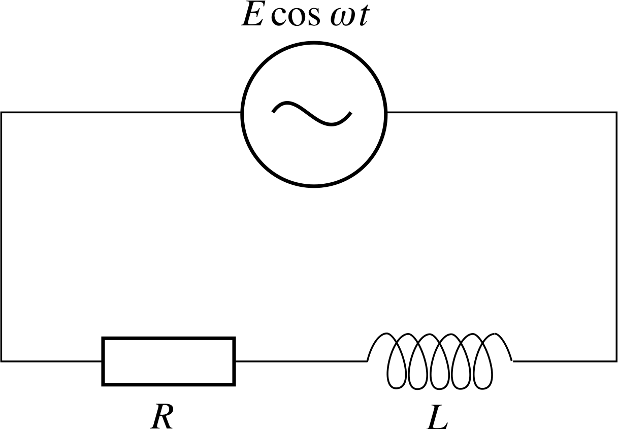
Figure 3 An electrical circuit containing a resistor, an inductor and an ideal voltage generator.
Electric current
The second example concerns the way in which the electric current I in the circuit shown in Figure 3 varies with time.
The circuit contains an inductor of inductance L, a resistor of resistance R, and an ideal voltage generator producing an alternating voltage E cos(ωt).
The differential equation determining the electric current I at time t is
$L\dfrac{dI}{dt} + RI = E\cos(\omega t)$(25)
The general approach
Look carefully at Equations 24 and 25 and convince yourself that they cannot be written in any of the three ways shown in Equations 1, 4 and 14,
$\dfrac{dy}{dx} = f(x)$(Eqn 1)
$\dfrac{dy}{dx} = h(y)$(Eqn 4)
$\dfrac{dy}{dx} = f(x)h(y)$(Eqn 14)
but that they are of the form shown in Equation 23,
$a\dfrac{dy}{dx} + by = f(x)$(Eqn 23)
The general method of solving equations such as Equation 23 is somewhat more complicated than the other methods we have studied in this module; so, on this occasion, let us start with a particular example that may make the general method easier to understand. If you are given the information that
y ex = sin x + C(26)
where C is a constant, you would be able to differentiate this equation with respect to x to obtain
${\rm e}^x\dfrac{dy}{dx} + {\rm e}^xy = \cos x$(27)
Therefore if we were asked to solve the Equation 27, we can see immediately that its general solution is the function y (x) given by Equation 26. But suppose that we alter the differential equation slightly by dividing both sides by ex to get
$\dfrac{dy}{dx} + y = {\rm e}^{-x}\cos x$(28)
The general solution remains the same, it is still y (x), but the left–hand side of Equation 28 is no longer the derivative of a simple function. If you were asked to solve Equation 28 you would need to multiply both sides of the equation by ex and then perhaps you might recognize that the left–hand side is the derivative of the product y ex. Having done that you would then only need to integrate the right–hand side, then perform some manipulations in order to find the general solution. This is the essence of the method, and its success will depend on choosing a suitable multiplier, in this case ex.
Now let us develop these ideas more systematically, in the context of our radioactive decay example, by trying to solve Equation 24,
$\dfrac{dN}{dt} + \lambda N = \mu B_0{\rm e}^{-\mu t}$(Eqn 24)
Perhaps by multiplying by some suitable function g (t) we can make the left–hand side the derivative of a product. Multiplying both sides of Equation 24 by h (t) we obtain
$h(t)\dfrac{dN}{dt} + \left[\lambda h(t)\right]N = \mu h(t)B_0{\rm e}^{-\mu t}$(29)
Now, the left–hand side of this equation would be the derivative of the product h (t)N (t) if the expression in square brackets was equal to dh/dt. In other words to make the left–hand side the derivative of a product we require
$\dfrac{dh}{dt} = \lambda h(t)$(30)
But Equation 30 is just a simple first–order differential equation that can be tackled by inversion and direct integration (as in Subsection 2.2). Its solution is
$\displaystyle t = \lambda \int \dfrac 1h\,dh = \dfrac{1}{\lambda}\loge h + C$(31)
We only need to find one function h (t) with the desired property, so we choose the simplest case, when C = 0, and Equation 31 then gives h (t) = eλt. Substituting this expression for h (t) in Equation 29 gives us
${\rm e}^{\lambda t}\dfrac{dN}{dt} + \lambda{\rm e}^{\lambda t}N = \mu{\rm e}^{\lambda t}B_0{\rm e}^{-\mu t}$
where the left–hand side is now clearly seen to be the derivative of the product N eλt with respect to t because we have constructed it to be so.
We can now see that
$\dfrac{d}{dt}\left(N{\rm e}^{\lambda t}\right) = \mu{\rm e}^{\lambda t}B_0{\rm e}^{-\mu t} = \mu B_0{\rm e}^{(\lambda-\mu)t}$
Integrating both sides gives us
$N{\rm e}^{\lambda t} = \dfrac{\mu B_0}{\lambda-\mu}{\rm e}^{(\lambda-\mu)t} + C$
Finally, if we make N the subject of this equation by dividing both sides by eλt we find
$N = \dfrac{\mu B_0}{\lambda-\mu}{\rm e}^{-\mu t} + C{\rm e}^{-\lambda t}$(32)
Question T7
Check by substitution that Equation 32 is a solution to Equation 24,
$\dfrac{dN}{dt} + \lambda N = \mu B_0{\rm e}^{-\mu t}$(Eqn 24)
Answer T7
Differentiating $N = \dfrac{\mu B_0}{\lambda-\mu}{\rm e}^{-\mu t} + C{\rm e}^{-\lambda t}$ with respect to t gives us
$\dfrac{dN}{dt} = \dfrac{\mu^2B_0}{\lambda-\mu}{\rm e}^{-\mu t} - \lambda C{\rm e}^{-\lambda t}$
and substituting this result, and the expression for N, into the left–hand side of Equation 24,
$\dfrac{dN}{dt} + \lambda N = \mu B_0{\rm e}^{-\mu t}$(Eqn 24)
gives us $\dfrac{dN}{dt} + \lambda N = \dfrac{\mu^2B_0 + \lambda\mu B_0}{\lambda-\mu}{\rm e}^{-\mu t} - \lambda C{\rm e}^{-\lambda t} = \mu B_0{\rm e}^{-\mu t}$
which is identical to the right–hand side of Equation 24. So Equation 32,
$N = \dfrac{\mu B_0}{\lambda-\mu}{\rm e}^{-\mu t} + C{\rm e}^{-\lambda t}$(Eqn 32)
is a solution to Equation 24.
It should be clear that this method would have worked whatever function of t had been present on the right–hand side of Equation 24,
$\dfrac{dN}{dt} + \lambda N = \mu B_0{\rm e}^{-\mu t}$(Eqn 24)
The important point of the technique is the trick of multiplying Equation 24 by eλt in order to bring its left–hand side into the form of Equation 27,
${\rm e}^x\dfrac{dy}{dx} + {\rm e}^xy = \cos x$(Eqn 27)
This was what made it possible to integrate directly, and for this reason, eλt is called an integrating factor.
An integrating factor is a function by which each term of a differential equation is multiplied in order to make it possible to use direct integration to solve the equation.
The general linear equation with constant coefficients
Now that we have found the integrating factor for Equation 24, we can easily find one for the general first–order linear equation with constant coefficients
$a\dfrac{dy}{dx} + by = f(x)$(Eqn 23)
If we divide both sides by the constant a, we obtain
$\dfrac{dy}{dx} + \dfrac ba y = \dfrac{f(x)}{a}$
The left–hand side here is just like the left–hand side of Equation 24,
$\dfrac{dN}{dt} + \lambda N = \mu B_0{\rm e}^{-\mu t}$(Eqn 24)
except that instead of λ we have the constant b/a. The following exercise shows that the integrating factor in thi case must be simply ebx/a, which can be written alternatively as exp(bx/a).
Question T8
Show that the following is true
$\dfrac{d}{dx}\left(y{\rm e}^{bx/a}\right) = {\rm e}^{bx/a}\dfrac{dy}{dx} + \dfrac ba y{\rm e}^{bx/a}$
and explain why this means that exp(bx/a) is the integrating factor for Equation 23.
Answer T8
If we use the product_rule_of_differentiationproduct rule of differentiation
$\dfrac{d}{dx}\left(y{\rm e}^{bx/a}\right) = {\rm e}^{bx/a}\dfrac{dy}{dx} + y\dfrac{d}{dx}\left({\rm e}^{bx/a}\right) = {\rm e}^{bx/a}\dfrac{dy}{dx} + \dfrac ba y{\rm e}^{bx/a}$
Thus if we multiply Equation 23,
$a\dfrac{dy}{dx} + by = f(x)$(Eqn 23)
by exp(bx/a), we obtain
$\dfrac{d}{dx}\left(y{\rm e}^{bx/a}\right) = {\rm e}^{bx/a}\dfrac{f(x)}{a}$
which can now be integrated directly. Hence exp(bx/a) is the integrating factor for Equation 23.
Question T9
Find the integrating factor for the following differential equation:
$2\dfrac{dy}{dx} - x = y$
Answer T9
If we divide both sides by 2 (and rearrange the equation so that all terms involving x are on the left–hand side) the equation becomes
$\dfrac{dy}{dx} - \dfrac12 y = \dfrac12 x$
It can then be seen that the integrating factor is exp(−x/2) in this case. Alternatively we can just use the formula eby/a with b = −1, a = 2 and y = x.
We will now summarize the steps involved in using the method of integrating factors to solve the first–order linear differential equation with constant coefficients,
$a\dfrac{dy}{dx} + by = f(x)$(Eqn 23)
Integrating factor method
- 1
-
Divide both sides of the equation by a, the coefficient of dy/dx, to obtain
$\dfrac{dy}{dx} + \dfrac ba y = \dfrac{f(x)}{a}$
- 2
-
Multiply both sides of the equation by ebx/a, the integrating factor. This gives
${\rm e}^{bx/a}\dfrac{dy}{dx} + \dfrac ba y{\rm e}^{bx/a} = f(x){\rm e}^{bx/a}$
which can be written as
$\dfrac{d}{dx}(y{\rm e}^{bx/a}) = {\rm e}^{bx/a}\dfrac{f(x)}{a}$
- 3
-
Integrate this equation directly, to obtain
$y{\rm e}^{bx/a} = \dfrac 1a {\displaystyle \int}f(x){\rm e}^{bx/a}\,dx$
- 4
-
Evaluate the integral, remembering to include the constant of integration.
- 5
-
If possible, make y the subject, by dividing all terms – including the constant of integration – by ebx/a.
- 6
-
Check that your answer is a solution by substitution.
You can now practise these six steps by answering the following questions.
Question T10
Use the integrating factor you found for the equation given in Question T9,
$2\dfrac{dy}{dx} - x = y$
to find the general solution of that equation.
Answer T10
Step 1 has already been performed in the answer to Question T9.
Step 2 Multiply both sides of the equation by exp(−x/2), the integrating factor found in Question T9, to give
$\dfrac{d}{dx}\left(y{\rm e}^{-x/2}\right) = \dfrac12 x{\rm e}^{-x/2}$
Step 3 Integrate this equation to give
$y{\rm e}^{-x/2} = \frac12 \Int x{\rm e}^{-x/2}\,dx$
Step 4 The integral can be evaluated by integrating by parts, to give
$y{\rm e}^{-x/2} = -x{\rm e}^{-x/2} - 2{\rm e}^{-x/2} + C$
Step 5 Make y the subject to give
y = −x − 2 + C ex/2
Question T11
Find the general solution to Equation 25,
$L\dfrac{dI}{dt} + RI = E\cos(\omega t)$(25)
You will need to use the following standard integral:
$\dfrac EL {\displaystyle \int}{\rm e}^{Rt/L}\cos(\omega t)\,dt = \dfrac{E}{R^2+L^2\omega^2}{\rm e}^{Rt/L}[\omega L\sin(\omega t) + R\cos(\omega t)] + C$
Answer T11
Step 1 Divide both sides of Equation 25,
$L\dfrac{dI}{dt} + RI = E\cos(\omega t)$(Eqn 25)
by L, to obtain
$\dfrac{dI}{dt} + \dfrac RL I = \dfrac EL \cos(\omega t)$
Step 2 Multiply both sides of the equation by the integrating factor exp(Rt/L) to give
$\dfrac{d}{dt}\left(I{\rm e}^{Rt/L}\right) = \dfrac EL {\rm e}^{Rt/L}\cos(\omega t)$
Step 3 Integrate both sides to give
$\displaystyle I{\rm e}^{Rt/L} = \dfrac EL \int{\rm e}^{Rt/L}\cos(\omega t)\,dt$
Step 4 The integral here is a standard integral; therefore
$I{\rm e}^{Rt/L} = \dfrac{E}{R^2+L^2\omega^2}\left[\omega L\sin(\omega t)+R\cos(\omega t)\right]{\rm e}^{Rt/L} + C$
Step 5 To make I the subject, divide both sides by eRt/L, to obtain
$I = \dfrac{E}{R^2+L^2\omega^2}\left[\omega L\sin(\omega t)+R\cos(\omega t)\right] + C{\rm e}^{-Rt/L}$
2.5 Choosing the correct method; what to do if none of them work
So far we have discussed differential equations of the following forms:
- 1
-
$\dfrac{dy}{dx} = f(x)$, which can be solved by direct integration;
- 2
-
$\dfrac{dy}{dx} = h(y)$, which can be solved by inversion and then direct integration;
- 3
-
$\dfrac{dy}{dx} = f(x)h(y)$, which can be solved by separation of variables;
- 4
-
$a\dfrac{dy}{dx}+ by = f(x)$, the linear equation with constant coefficients, which can be solved by means of an integrating factor.
When faced with a first–order differential equation, you should first see whether it can be written in any of the above four forms (making sure that you have correctly identified the independent and dependent variables); if it can, you should then use the appropriate method to find its general solution.
The following exercise is intended to test your ability to choose the appropriate method (you are not asked to solve the differential equations).
Question T12
What method would you use to solve the following differential equations? (In some cases, more than one method is possible; but you should not use separation of variables if direct integration or inversion and direct integration would work.)
(a) $y\dfrac{dy}{dx} = \dfrac{1}{x^2} + \dfrac{y^2}{x^2}$
(b) $\dfrac{dv}{dt} = -g + \dfrac{\alpha}{\beta-\gamma t}$ where g, α, β and γ are constants.
(c) $\dfrac{dy}{dx} = 5(y+3x)$
(d) $\dfrac{dN}{dt} + \lambda N = R$ where λ and R are constants.
Answer T12
(a) Separation of variables; the equation can be written as
$\dfrac{dy}{dx} = \dfrac{1+y^2}{y}\times \dfrac{1}{x^2}$
(b) Direct integration (the right–hand side is a function of t and constants only).
(c) This is a linear equation which can be solved by means of an integrating factor.
(d) This is also a linear equation, so could be solved by finding an integrating factor; alternatively, it can be
solved by inversion and integration.
Change of variable
There are, of course, many first–order differential equations that cannot be written in any of the forms 1 to 4 above. Sometimes, however, an equation of that sort can be transformed into one that we already know how to solve by changing the (dependent) variable. The best way to explain this technique is by means of an example.
Consider the differential equation
$\dfrac{dy}{dx} = \dfrac yx + \dfrac xy$(33) i
This equation is neither separable nor linear. However, let us see what happens if we define a new dependent variable v in terms of y and x by
y = vx, which can be rewritten as v = y/x(34)
where v is to be regarded as a (so far unknown) function of x. Since y = vx we can use the product rule to obtain the following expression for the left–hand side of Equation 33,
$\dfrac{dy}{dx} = \dfrac{d}{dx}(vx) = x\dfrac{dv}{dx} + v$
We can now use Equation 34 to rewrite the right–hand side of Equation 33 in the following way
$\dfrac yx + \dfrac yx = v + \dfrac 1v$
Using these results Equation 33 becomes
$x\dfrac{dv}{dx} + v = v + \dfrac 1v$
that is $x\dfrac{dv}{dx} = \dfrac 1v$
which can be separated and integrated to obtain
${\displaystyle \int}\dfrac 1x\,dx = \Int v\,dv$
giving $\loge x + C = \frac 12 v^2$
Rearranging this equation to make v the subject, we find:
$v = \pm\sqrt{2\loge x + C_1\os}$
(where the new constant C1 = 2C). Finally, we express the solution in terms of our original independent variable, by putting v = y/x, to obtain the general solution
$y = \pm x\sqrt{2\loge x + C_1\os}$
There is no systematic way of finding a change of variable that will convert an otherwise insoluble differential equation into one that can be solved by one of the techniques you have learnt in this module. Often it is necessary to proceed simply by trial and error, though we can give you one hint: if the equation contains a particular combination of the variables y and x, it is worth seeing what happens if you make that combination your new dependent variable. (That was why we tried y = vx in Equation 33;
$\dfrac{dy}{dx} = \dfrac yx + \dfrac xy$(Eqn 33)
the right–hand side is simply a function of y/x.)
Question T13
Show that the differential equation
$\dfrac{dy}{dx} = \dfrac{1}{(y + x)^2}$
can be converted into an equation that can be solved by inversion by means of the change of variable v = y + x. (You are not required to find the solution.)
Answer T13
If v = y + x, so that y = v − x, then dy/dx = dv/dx − 1. Substituting this, and y + x = v, into the differential equation gives us
$\dfrac{dv}{dx} = 1 + \dfrac{1}{v^2}$
As the right–hand side here is a function only of v the (new) dependent variable, the equation can be solved by inversion and integration.
As you become more experienced in solving differential equations, you will find it easier to spot the change of variable that makes the equation soluble, if there is one (there may not be; for example, we know of no change of variable that makes it possible to solve the equation dy/dx = y x).
Of course, you can always seek help from textbooks, which often discuss changes of variable that will work for particular types of differential equations. You should regard a differential equation that cannot be solved by any of the four systematic methods listed above as an interesting challenge; it is, after all, at this point that the process of solving differential equations ceases simply to be a routine matter of applying standard technique and becomes something of an art, requiring ingenuity, patience and low animal cunning.
3 Closing items
3.1 Module summary
- 1
-
Subsection 2.1First-order differential equations of the form dy/dx = f (x) can be solved at once by direct integration, to give $y = \Int f(x)\,dx$.
- 2
-
Equations of the form dy/dx = h (y) can be solved by applying the inversion rule, dy/dx = 1/(dx/dy), to obtain dx/dy = 1/h (y), which can be directly integrated.
- 3
-
Equations of the form dy/dx = f (x)h (y) can be solved by the technique of separation of variables, which leads to an equation of the form
$\displaystyle \int\dfrac{1}{h(y)}\,dy = f(x)\,dx$(Eqn 18)
which may be integrated and rearranged to find y.
- 4
-
Linear first–order differential equations with constant coefficients of the form a (dy/dx) + by = f (x) can be solved by dividing both sides by a and then multiplying both sides by an integrating factor exp(bx/a), to bring them into a form where direct integration becomes possible.
- 5
-
The technique of changing the dependent variable is almost the only option available if none of the methods listed above works. This is a trial and error procedure rather than a systematic one.
3.2 Achievements
Having completed this module, you should be able to:
- A1
-
Define the terms that are emboldened and flagged in the margins of the module.
- A2
-
Solve differential equations of the form dy/dx = f (x), by direct integration.
- A3
-
Use the inversion rule to solve differential equations of the form dy/dx = h (y), by inversion and direct integration.
- A4
-
Explain what is meant by the term separable, and solve differential equations of the form dy/dx = f (x)h (y), by separation of variables.
- A5
-
Explain what is meant by an integrating factor, find the integrating factor for a linear first–order equation with constant coefficients and use it to solve the equation.
- A6
-
Decide which (if any) of the above methods can be used to solve a given first–order differential equation.
- A7
-
Use a given change of variable to transform a first–order differential equation into one that can more easily be solved.
Study comment You may now wish to take the following Exit test for this module which tests these Achievements. If you prefer to study the module further before taking this test then return to the topModule contents to review some of the topics.
3.3 Exit test
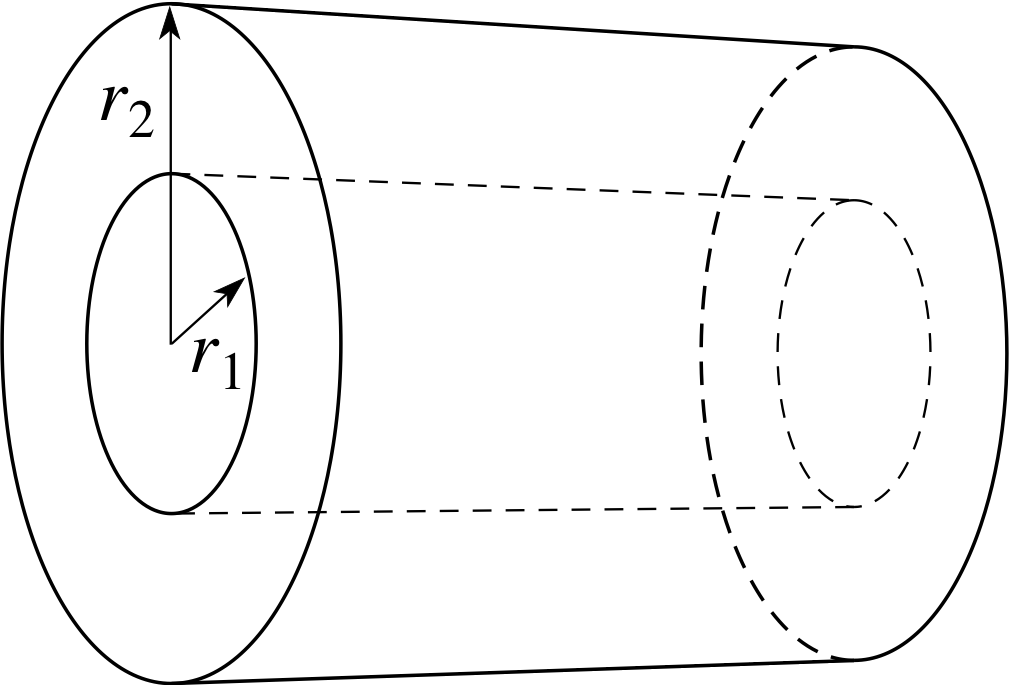
Figure 4 See Question E1.
Question E1 (A2)
The differential equation
$H = -2\pi r\kappa\dfrac{dT}{dr}$
describes the way in which temperature T varies with radius r within the walls of a hollow cylindrical pipe, of inner radius r1 and outer radius r2 (see Figure 4). H (the heat loss per unit length) and κ (the thermal conductivity of the pipe) are constants. Find the general solution of this equation by direct integration.
If the temperature of the inner wall is T1, find an expression for the temperature T2 of the outer wall in terms of T1, r1, r2 and constants.
Answer E1
Rearranging the equation so that it can be integrated directly gives us
$\dfrac{dT}{dr} = -\dfrac{H}{2\pi r\kappa}$
so that$T = -\dfrac{H}{2\pi\kappa}{\displaystyle \int}\dfrac{dr}{r} = -\dfrac{H}{2\pi\kappa}\loge(r/C)$
Note that in this case we have introduced the integration constant (which will have the same dimensions as r) into the argument of the logarithmic function to ensure that it is dimensionless. This is always possible since in general terms
loge (x/A) = loge x + loge A = loge x + B
At r = r1, T = T1; substituting this into the general solution gives us
$T_1 = -\dfrac{H}{2\pi\kappa}\loge(r_1/C) = \dfrac{H}{2\pi\kappa}\loge(C/r_1)$
so that, after a little manipulation, the particular solution can be written as
$T = T_1 - \dfrac{H}{2\pi\kappa}\loge(r/r_1)$
Thus at r = r2, the temperature T2 is
$T_2 = T_1 - \dfrac{H}{2\pi\kappa}\loge(r_2/r_1)$
(Reread Subsection 2.1 if you had difficulty with this question.)
Question E2 (A3)
Use the technique of inversion and integration to find the general solution to the differential equation
$\dfrac{dy}{dx} = \sqrt{a^2 - y^2}$ where a is a constant
Answer E2
Inverting the equation gives us $\dfrac{dx}{dy} = \dfrac{1}{\sqrt{a^2-y^2}}$
By integrating, we obtain the standard integral
$\displaystyle x = \int\dfrac{1}{\sqrt{a^2-y^2}} = \arcsin(y/a) + C$
Making y the subject, gives us the general solution
y = a sin(x − C)
(Reread Subsection 2.2 if you had difficulty with this question.)
Question E3 (A4)
The following equation describes how the (absolute) temperature T at which a liquid boils varies with the external pressure P (under certain assumptions, which we shall not go into here):
$\dfrac{dT}{dP} = \dfrac{RT^2}{LP}$
where L (the molar latent heat of vaporization of the liquid) and R (the molar gas constant) are constants.
Find the general solution to this equation using the technique of separation of variables.
Answer E3
Separating variables here gives us
$\displaystyle \int\dfrac{1}{T^2}\,dT = \dfrac RL \int\dfrac 1P\,dP$
On evaluating the integrals, we obtain
$-\dfrac 1T = \dfrac RL \loge(P/C)$
(Notice that once again we have introduced the integration constant into the logarithmic function’s argument to make it dimensionless, rather than writing the less satisfactory (R/L) loge P + constant.)
If we make T the subject, we find the general solution
$T = -\dfrac{L}{R\loge(P/C)}$
(Reread Subsection 2.3 if you had difficulty with this question.)
Question E4 (A3 and A5)
A stone of mass m is thrown vertically upwards with initial velocity ux. The stone is subject to the (downward) force of gravity, of magnitude −mg, and a resistive force of magnitude −mkvx (where k is a positive constant), the stone’s upward velocity vx at time t satisfies the differential equation
$\dfrac{dv_x}{dt} = -g - kv_x$ (vx > 0)
Find the general solution to this equation:
(a) by using inversion and direct integration (treating the cases when (g + kvx) is positive and negative separately); and
(b) by using an integrating factor.
(c) Use the initial condition vx = ux at t = 0 to find the particular solution.
Answer E4
(a) Inverting the equation gives us
$\dfrac{dt}{dv_x} = -\dfrac{1}{g+kv_x}$ (for vx ≠ −g/k)
We treat the two cases g + kvx > 0 (i.e. vx >− g/k) and g + kvx < 0 (i.e. vx < −g/k) separately in evaluating the integral.
If g + kvx > 0, then
$\displaystyle t = -\int\dfrac{1}{g+kv_x}\,dv_x = -\dfrac 1k\loge[(g + kv_x)/C]$
On making vx the subject, we obtain
vx = C e−kt − g/k
where C is a positive constant.
If g + kvx < 0, then
$\displaystyle t = -\int\dfrac{1}{g+kv_x}\,dv_x = -\dfrac 1k\loge[-(g + kv_x)/C]$
On making vx the subject, we obtain
vx = −C e−kt − g/k
where C is a positive constant.
By inspection, vx = −g/k is a particular solution. Thus the general solution is
vx = D e−kt − g/k
where the arbitrary constant D may be positive, negative or zero.
(b) Writing the equation as $\dfrac{dv_x}{dt} + kv_x = -g$, we see that the integrating factor is exp(kt).
On multiplying both sides of the equation by this, the differential equation becomes
$\dfrac{d}{dt}\left(v_x{\rm e}^{kt}\right) = -g{\rm e}^{kt}$
and we may now integrate, to obtain
$v_x{\rm e}^{kt} = -g\Int{\rm e}^{kt}\,dt = -\dfrac gk {\rm e}^{kt} + C$
Multiplying throughout by e−kt gives us
vx = C e−kt − g/k
as we found in part (a). (Note this is not the same C as in part (a).)
(c) If we use the initial condition, vx = ux at t = 0 in the general solution we obtain ux = C − g/k, or C = ux + g/k. So the particular solution can be written as
$v_x = \left(u_x + \dfrac gk\right){\rm e}^{-kt} - \dfrac gk$
(Reread Subsection 2.2Subsections 2.2 and Subsection 2.42.4 if you had difficulty with this question.)
Question E5 (A6)
Find the general solutions of the following differential equations:
(a) $\dfrac{du}{dT} = 4\dfrac uT$ where u and T are both always positive.
(b) $R\dfrac{dQ}{dt} + \dfrac{Q}{C_0} = E{\rm e}^{-\lambda t}$ where R, C0, E and λ are constants.
Answer E5
(a) This equation is separable. On separating variables, we obtain
$\displaystyle \int \dfrac1u\,du = 4\int\dfrac1T\,dT$
and evaluating the integral gives us
$\loge u = 4\loge T + C$
Making u the subject we find u = C1T 4, where C1 = exp C is an arbitrary constant.
(b) This is a linear equation. Dividing both sides of the equation by R gives us
$\dfrac{dQ}{dt} + \dfrac{Q}{RC_0} = \dfrac ER{\rm e}^{-\gamma t}$
so that the integrating factor is exp(t/RC0). Multiplying the above equation by this factor brings it to the form
$\dfrac{d}{dt}\left(Q{\rm e}^{t/RC_0}\right) = \dfrac ER{\rm e}^{t/RC_0}{\rm e}^{-\gamma t}$
which may be integrated to give
$\displaystyle Q{\rm e}^{t/RC_0} = \dfrac ER\int{\rm e}^{t/RC_0}{\rm e}^{-\gamma t}\,dt = \dfrac{EC_0}{1-\lambda RC_0}{\rm e}^{t/RC_0}{\rm e}^{-\gamma t} + C$
Making Q the subject of this equation by dividing both sides by et/RC0 gives us
$Q = \dfrac{EC_0}{1-\lambda RC_0}{\rm e}^{-\gamma t} + C{\rm e}^{-t/RC_0}$
(Reread Subsection 2.3Subsections 2.3 and Subsection 2.42.4 if you had difficulty with this question.)
Question E6 (A4, A5, A6 and A7)
A differential equation of the form
$\dfrac{dy}{dx} + y = f(x)y^n$
where n is a constant (not necessarily an integer), is called a Bernoulli equation.
(a) For one value of n, the equation is linear with constant coefficients. What is this value?
(b) For another value of n, the equation is separable. What is this value?
(c) If n is not equal to either of these two values, the equation cannot be solved as it stands. Show that the substitution y = v m, where m = 1/(1 − n), transforms the equation into a linear equation.
(d) Find the general solution of the equation if n = 2 and f (x) = e2x.
Answer E6
(a) The equation is linear with constant coefficients if n = 0.
(b) The equation is separable if n = 1.
(c) If y = vm, then $\dfrac{dy}{dx} = mv^{m-1}\dfrac{dv}{dx}$ and y n = vmn.
Substituting these two expressions into the equation gives us
$mv^{m-1}\dfrac{dv}{dx} + v^m = f(x)v^{mn}$
Dividing both sides by vm−1 gives us
$m\dfrac{dv}{dx} + v = f(x)v^{mn-m+1}$
so that if m = 1/(1 − n), then mn − m + 1 = 0, and v disappears from the rig right–hand, leaving us with a linear equation with constant coefficients:
$m\dfrac{dv}{dx} + v = f(x)$
or, if we put m = 1/(1 − n)
$\dfrac{dv}{dx} + (1-n)v = (1-n)f(x)$
(d) If n = 2 and f (x) = exp(2x), we can make the change of variable y = 1/v (since m = 1/(1 − n) = −1 here). Then the equation becomes
$\dfrac{dv}{dx} - v = {\rm e}^{2x}$
The integrating factor is exp(−x); on multiplying the equation by this factor we obtain
$\dfrac{d}{dx}\left(v{\rm e}^{-x}\right) = -{\rm e}^x$
Integration gives $v{\rm e}^{-x}= -\Int{\rm e}^x\,dx = -{\rm e}^x + C$, and on making v the subject, we find $v = -{\rm e}^{2x} + C{\rm e}^x$.
Since v = 1/y the general solution for y is
y = (−e2x + C ex)−1
(Reread Subsection 2.3Subsections 2.3, Subsection 2.42.4 and Subsection 2.52.5 if you had difficulty with this question.)
Study comment This is the final Exit test question. When you have completed the Exit test go back and try the Subsection 1.2Fast track questions if you have not already done so.
If you have completed both the Fast track questions and the Exit test, then you have finished the module and may leave it here.
Study comment Having completed this module, you should be able to answer the following questions each of which tests one or more of the Achievements.
Many of the questions in the Exit test involve the evaluation of an indefinite integral as one of the steps. In the solutions, a detailed explanation of how the integral is to be evaluated is not given. If you have trouble with any of these integrals, you should consult the Glossary, or one of the modules dealing with integration.