MATH 5.4: Applications of integration |
PPLATO @ | |||||
PPLATO / FLAP (Flexible Learning Approach To Physics) |
||||||
|
1 Opening items
1.1 Module introduction
You probably know that the volume of a sphere of radius r is $\frac43\pi r^3$, but do you know how to prove that this is the case? One way to proceed is to divide the sphere into a set of thin discs, to find an approximate expression for the volume of each disc, then add all the approximations, and so estimate the volume of the sphere. As we allow the discs to get thinner and thinner, the accuracy of the approximation improves and approaches a limiting value – the limit of a sum – which is usually known as a definite integral.
This module discusses several physical and geometrical applications of integration, all based on the fact that a definite integral is the limit of an appropriate sum. This idea is probably already familiar to you, since you may well have been introduced to definite integrals in the context of calculating areas under graphs, where such an area is approximated by a set of thin rectangles. However, the module starts with a review of the relation between a definite integral and an area, and discusses cases where the area actually corresponds to some physical quantity. It goes on to show how definite integrals can be used to find more complicated areas those enclosed by two intersecting graphs. Then it discusses some examples of solids (solids of revolution) whose volumes and surface areas can be written as definite integrals. (Here, you will find a derivation of the formula for the volume of a sphere.) Finally, it shows you how to express several other quantities masses of objects whose density is not constant, centres of mass and moments of inertia of solid objects, average values as definite integrals.
Study comment Having read the introduction you may feel that you are already familiar with the material covered by this module and that you do not need to study it. If so, try the following Fast track questions. If not, proceed directly to the Subsection 1.3Ready to study? Subsection.
1.2 Fast track questions
Study comment Can you answer the following Fast track questions? If you answer the questions successfully you need only glance through the module before looking at the Subsection 5.1Module summary and the Subsection 5.2Achievements. If you are sure that you can meet each of these achievements, try the Subsection 5.3Exit test. If you have difficulty with only one or two of the questions you should follow the guidance given in the answers and read the relevant parts of the module. However, if you have difficulty with more than two of the Exit questions you are strongly advised to study the whole module.
Question F1
Find the area of the region bounded by the graph of the function y = x2 + 2 and the line y = 5 − 2x.
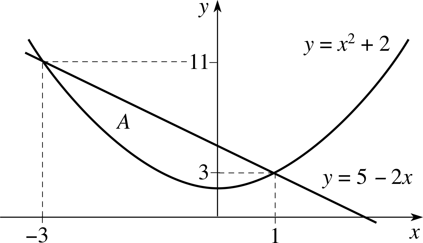
Figure 27 See Answer F1.
Answer F1
We first find the points of intersection of the two graphs, and sketch the region whose area has to be found. The points of intersection occur where x2 + 2 = 5 − 2x or x2 + 2x − 3 = 0, and the roots of this quadratic equation are x = −3 and x = 1. The graphs are sketched in Figure 27.
Since the graph of the line y = 5 − 2x lies above the graph of y = x2 + 2 over the interval −3 ≤ x ≤ l, we integrate the function (5 − 2x) − (x2 + 2) = 3 − 2x − x2 over this interval to obtain the area A which is, therefore,
$A = {\large\int}_{-3}^1\left(3-2x-x^2\right)\,dx = \left[3x-x^2-\frac13x^3\right]_{-3}^1 = 1.667 - (-9) = 10.667$
Question F2
Given that the integral $\Int_0^1\sqrt{1 + u^2}\,du = 1.14779$, find, to two decimal places, the area of the surface of revolution generated by the graph of y = sin x as it is rotated about the x–axis over the interval 0 ≤ x ≤ π/2.
Answer F2
The area of the surface of revolution generated by the curve y = f (x) over the interval a ≤ x ≤ b is
$S = 2\pi{\large\int}_a^bf(x)\sqrt{1+\left[\,f'(x)\right]^2}\,dx$
Here, f (x) = sin x, so f ′ (x) = cos x; and the region of integration is 0 ≤ x ≤ π/2. Hence
$S = 2\pi{\large\int}_0^{\pi/2}\sin x\sqrt{1+\cos^2x}\,dx$
We make the substitution u = cos x; then du = −sin x dx. When x = 0, u = 1 and when x = π/2, u = 0, so
$S= -2\pi{\large\int}_1^0\sqrt{1+u^2}\,du = 2\pi{\large\int}_0^1\sqrt{1+u^2}\,du = 2\pi \times 1.14779 = 7.21$
Question F3
A circular disc has radius a, mass M and thickness t, and its density at any point is proportional to the distance of that point from the axis of the disc (i.e. the line perpendicular to the plane of the disc and through its centre). Find the moment of inertia of the disc about its axis. Express your answer in terms of M and a.
Answer F3
We divide the disc into rings, of width ∆r. The moment of inertia about the given axis of one such ring of average radius r is
$\underbrace{\underbrace{2\pi rt\,\Delta r\us}_{\color{purple}{\large\text{ volume }}}\underbrace{\rho(r)\us}_{\color{purple}{\large\text { density }}}}_{\color{purple}{\large\text{mass}}}\underbrace{r^2\us}_{\color{purple}{\large\substack{\text{distance}\\[1pt]\text{from axis}\\[1pt]\text{squared}}}} $
where ρ (r) is the density of the disc at distance r from the centre. So the total moment of inertia I is given by the integral $I = 2\pi t{\large\int}_0^ar^3\rho(r)\,dr$. We are told that ρ (r) = kr, where k is a constant. Thus
$I = 2\pi t{\large\int}_0^akr^4\,dr = 2\pi tk\left[\frac15r^5\right]_0^a = \frac25\pi tka^5$
But we want an answer in terms of M and a, not k, t and a. So we must express kt in terms of M and a, by calculating the mass of the disc. The mass of a ring is 2πrtρ (r) ∆r, so
$M = 2\pi tr{\large\int}_0^a\rho(r)\,dr = 2\pi tkr^2\,dr = 2\pi tk\left[\frac13r^3\right]_0^a = \frac23\pi tka^3$
Comparing this with the expression obtained for I, we see that $\dfrac IM = \frac35a^2$; so $I = \frac35Ma^2$.
1.3 Ready to study?
Study comment In order to study this module, you will need to be familiar with the following terms: centre of mass, definite integral, improper integral, integrand, integration by parts, integration by substitution, limits of integration, modulus, moment of inertia, range of integration. If you are uncertain of any of these terms, you can review them now by referring to the Glossary which will indicate where in FLAP they are developed. In addition, you will need to be familiar with various trigonometric identities, and you should know how to find standard integrals (such as the integrals of x n, or eax), and to evaluate definite integrals by the method of integration_by_substitutionsubstitution, or by integration by parts. You will also need to be able to sketch graphs of straight lines, quadratic_equationquadratic and cubic_equationcubic polynomial_expressionpolynomials, reciprocal functions, circles and ellipses; and know how to find the intersectpoints of intersection of two graphs. The following questions will allow you to establish whether you need to review some of these topics before embarking on this module.
Question R1
Evaluate the definite integrals
(a) $\Int_2^4(3x^5-16x^3)\,dx$ (b)$\Int_1^2\sqrt{4-x\os}\,dx$ (c)$\displaystyle \int_{a/2}^a\dfrac{1}{a^2-x^2}\,dx$
Answer R1
(a) $\Int(3x^5-16x^3)\,dx = \left[\frac12x^6-4x^4\right]_2^4 = 1024 - (-32) = 1056$
(b) This integral may be evaluated by the integration_by_substitutionsubstitution u = 4 − x. Then du = −dx and the integrand is equal to $\sqrt{u\os}$. When x = 1, u = 3, and when x = 2, u = 2, so the new limits of integration are 3 and 2. Thus
$\displaystyle \int_1^2\sqrt{4-x\os}\,dx = -\int_3^2\sqrt{u\os}\,dx = \int_2^3\sqrt{u\os}\,dx = \left[\frac23u^{3/2}\right]_2^3 = \frac23(5.196 - 2.828) = 1.578$
(c) This integral may be evaluated by the integration_by_substitutionsubstitution x = a sin u. Then $\sqrt{a^2-x^2} = a\cos u$ and dx = a cos u du.
When x = a, sin u = 1, so u = π/2, and when x = a/2, $\sin u = \frac12$, so u = π/6. Thus
${\displaystyle \int}_{a/2}^a\dfrac{1}{\sqrt{a^2-x^2}}\,dx = \Int_{\pi/6}^{\pi/2}\,du = {\large[}u{\large]}_{\pi/6}^{\pi/2} = \dfrac{\pi}{2}-\dfrac{\pi}{6} = \dfrac{\pi}{3}$
Question R2
Find the integral $\Int_0^Rx{\rm e}^{-ax}\,dx$, where a and R are positive constants. Hence find the improper integral $\Int_0^\infty x{\rm e}^{-ax}\,dx$
Answer R2
This integral can be evaluated using the formula for integration by parts
$\Int_a^bf(x)g(x)\,dx = \left[F(x)g(x)\right]_a^b - \Int_a^bF(x)\dfrac{dg}{dx}\,dx$
where dF/dx = f (x). Taking f (x) = e−ax, g (x) = x, we have $F(x) = -\dfrac1a{\rm e}^{-ax}$ and $\dfrac{dg}{dx} = 1$. So
$\Int_0^Rx{\rm e}^{-ax}\,dx = \left[-\dfrac1ax{\rm e}^{-ax}\right]_0^R + \dfrac1a\Int_0^R{\rm e}^{-ax}\,dx = \left[-\dfrac1ax{\rm e}^{-ax}\right]_0^R + \dfrac1a\left[-\dfrac1a{\rm e}^{-ax}\right]_0^R = -\dfrac Ra{\rm e}^{-ax} - \dfrac1a{\rm e}^{-ax} + \dfrac{1}{a^2}$
To find the improper integral $\Int_0^\infty x{\rm e}^{-ax}\,dx$, we let the upper limit R tend to infinity. As R becomes very large, both e−ax and Re−ax become very small (since a > 0), and their limit as R tends to infinity is zero. So
$\Int_0^\infty x{\rm e}^{-ax}\,dx = 1/a^2$
Question R3
Sketch the graphs of (a) y = x3 − 4x, (b) (x − 3)2 + (y + 1)2 = 9.
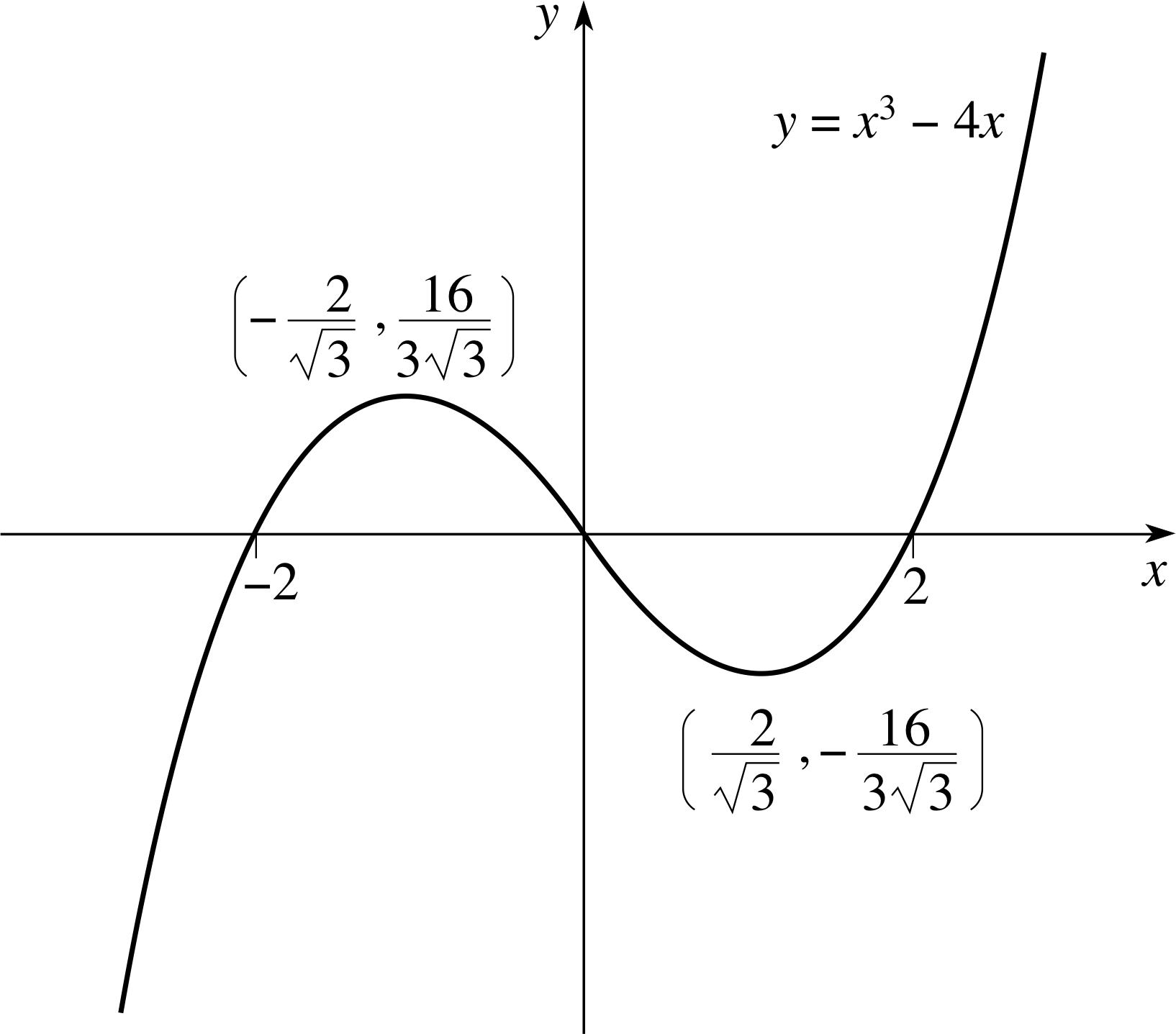
Figure 28 See Answer R3(a).
Answer R3
(a) The sketch is shown in Figure 28. The function crosses the x–axis where x2 −4x = 0, or x (x2 − 4) = 0, i.e. at x = 0, x = −2 and x = 2.
It has stationary points where $\dfrac{d}{dx}(x^3-4x) = 0$, or 3x2 − 4 = 0, i.e. at $x = 2/\sqrt{3\os}$ (where $y = -16/(3\sqrt{3\os})$; this turning point is a minimum) and at $x = -2/\sqrt{3\os}$, (where $y = 16/(3\sqrt{3\os})$, this turning point is a maximum).
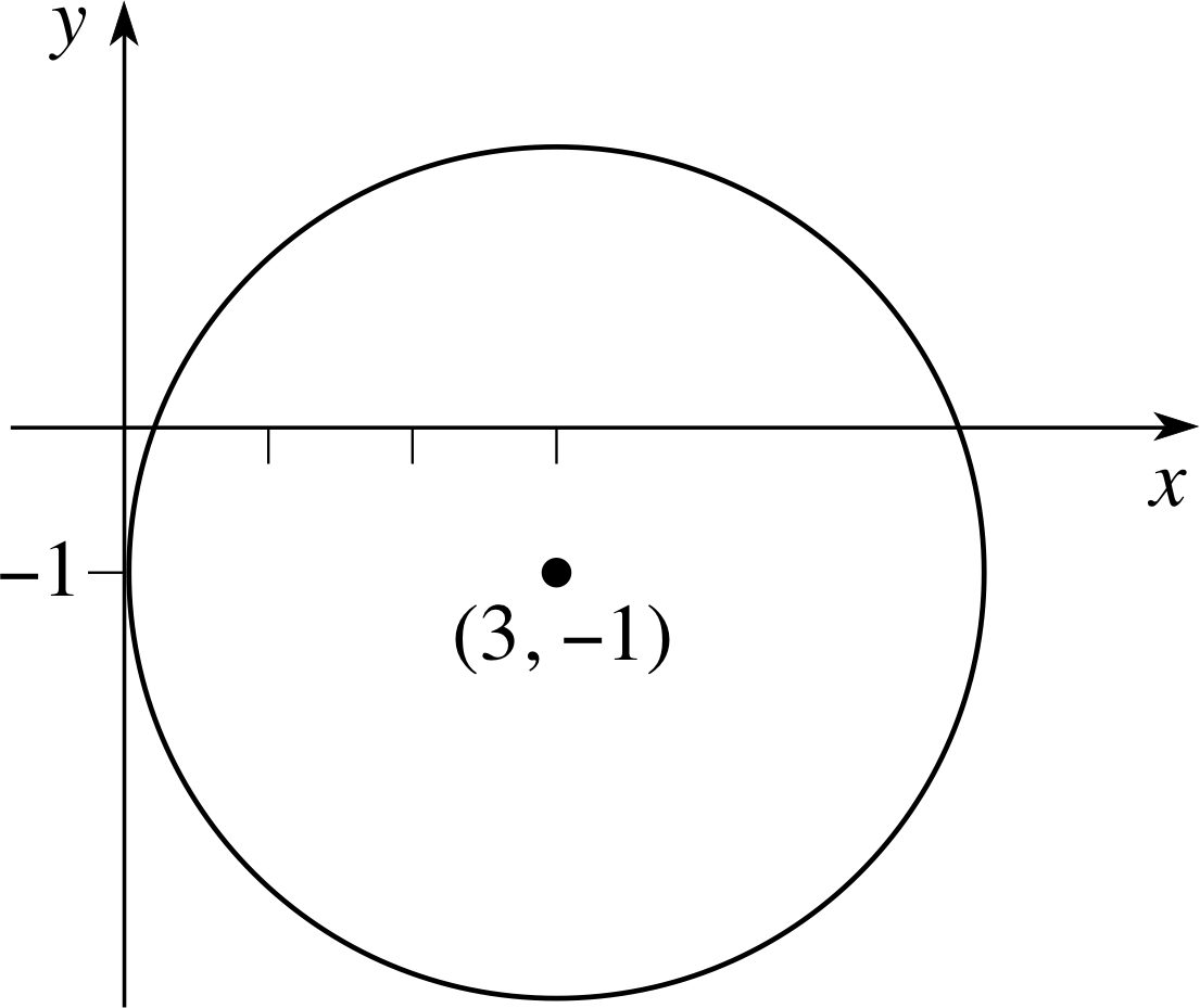
Figure 29 See Answer R3(b).
(b) This graph is a circle, with centre (3, −1) and radius 3; see Figure 29.
Question R4
Find the points of intersection of the line y = x − 3 with the graph of y = x2 − 5x + 4, and sketch these two functions on the same axes.
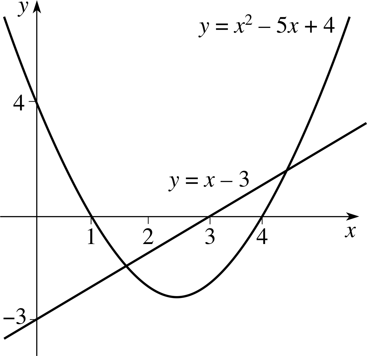
Figure 30 See Answer R4.
Answer R4
The points of intersection of the two graphs have x–coordinates satisfying the equation x − 3 = x2 − 5x + 4, or x2 − 6x + 7 = 0. This quadratic equation has solutions $x = 3\pm\sqrt{2\os}$. When $x = 3+\sqrt{2\os}$, $y = \sqrt{2\os}$ and when $x = 3-\sqrt{2\os}$, $y = -\sqrt{2\os}$. So the points of intersection are $(3 + \sqrt{2\os},\,\sqrt{2\os})$ and $(3 - \sqrt{2\os},\,-\sqrt{2\os})$, i.e. (4.41, 1.41) and (1.59, −1.41).
The line y = x − 3 has y–intercept −3, and crosses the x–axis at x = 3. The parabola y = x2 − 5x + 4 crosses the x–axis where x2 − 5x + 4 = 0; the solutions to this equation are x = 4 and x = 1. It crosses the y–axis at y = 4.
The two graphs are sketched in Figure 30.
Question R5
Two small objects, of masses 0.1 kg and 0.2 kg, are 1 m apart. Find (a) the position of their centre of mass; (b) their moment of inertia about an axis which passes through their centre of mass and is perpendicular to the line joining them.
Answer R5
(a) The centre of mass lies along the line joining the two objects. If the objects have masses m1 and m2 and are located at positions (x1, 0) and (x2, 0), respectively, then their centre of mass is at (xc, 0) where $x_{\rm c} = \dfrac{m_1x_1 + m_2x_2}{m_1 + m_2}$. We may take the object of mass m2 = 0.1 kg to be at the origin, so x1 = 0; then the object of mass m2 = 0.2 kg is at x2 = 1 m. So
$x_{\rm c} = \dfrac{(0.1\times 0) + (0.2\times 1)}{0.1 + 0.2}\,{\rm m} = 0.667\,{\rm m}$
i.e. the centre of mass lies between the two objects, and is 0.667 m from the object of mass 0.1 kg.
(b) The moment of inertia is defined as $\displaystyle I = \sum_{i=1}^Nm_ir_i^2$, where ri is the perpendicular distance of the object of mass mi from the axis. Here, r1 = 0.667 m and r2 = (1 − 0.667) m = 0.333 m. So
I = (0.1 kg) × (0.667 m)2 + (0.2 kg) × (0.333 m)2 = 6.67 × 10⁻² kg m2.
Question R6
In answering this question, you should make use only of trigonometric identities; you should not use your calculator.
(a) If $\cos\theta = \frac23$, what are the possible values of sin θ?
(b) If $\sin\theta = \frac13$, what is the value of cos(2θ)?
Answer R6
(a) If $\cos\theta = \frac23$ then we may use the identity cos2 θ + sin2 θ = 1 to deduce that $\sin^2\theta = 1 - \frac49 = \frac59$, so that $\sin\theta = \pm 5/\sqrt{3\os}$.
(b) If $\sin\theta = \frac13$ then we may use the identity cos(2θ) = 1 − 2 sin2 θ to obtain $\cos(2\theta) = 1 - \frac29 = \frac79$.
If you feel unsure about any of the terms used in Questions R1 to R6, consult the Glossary.
2 Areas
2.1 Area under a graph
You already know that a definite integral $\Int_a^bf(x)\,dx$ i can be related to an ‘area under the graph’ of the function f (x). If f (x) is a function that is positive over the interval a ≤ x ≤ b, then the integral$\Int_a^bf(x)\,dx$ is equal to the magnitude of the area enclosed by the graph of the function f (x), the vertical lines x = a and x = b, and the x–axis (see Figure 1). The area of this region is known as the ‘area under the graph’ of f (x) over the interval a ≤ x ≤ b. It is worth recalling here the argument that relates the definite integral $\Int_a^bf(x)\,dx$ to the area A shown in Figure 1, since we shall be using the same line of reasoning in many different cases throughout this module.
✦ Find the area under the graph of f (x) = x3 from x = 1 to x = 3. (Note: In this subsection we assume that both x and f (x) are dimensionless quantities.)
✧ The function f (x) = x3 is positive for all values of x in the interval 1 ≤ x ≤ 3, and so the required area is given by
${\large\int}_1^3x^3\,dx = \left[\dfrac14x^4\right]_1^3 = \dfrac14(81-1) = 20$ i
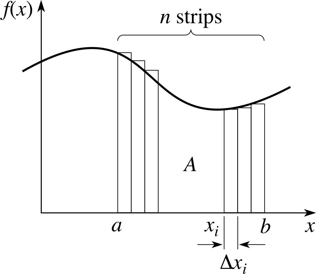
Figure 2 An approximation to the area under the graph of f (x).
The idea is that we can estimate a value for A by dividing the area up into a large number of thin rectangles. In Figure 2, the area under the graph of f (x) between x1 = a and xn+1 = b has been divided into n strips (although we only show six of them) which are then approximated by rectangles: the first is of height f (x1) and width ∆x1, the second is of height f (x2) and width ∆x2, and so on. The area of the ith rectangle, covering the interval [xi, xi + ∆xi] is f (xi) ∆xi and the sum of the areas of all these rectangles provides a good approximation to A, in other words,
$\displaystyle A \approx \sum_{i=1}^n f(x_i)\,\Delta x_i$(1) i
As we allow the width of the rectangles to become smaller and smaller (while, as a consequence, n gets larger) the sum on the right–hand side of Equation 1 becomes an ever better approximation to A, and in the limit, the sum is actually equal to A.
This limit of a sum is defined to be the definite integral $\Int_a^bf(x)\,dx$, so that we have
$A = \Int_a^bf(x)\,dx$(2)
The ‘area under a graph’ and the ‘magnitude of the area bounded by a graph’
In the above discussion we assumed that the function f (x) is positive between a and b, and we will need to make a minor adjustment if f (x) is negative or changes sign in the interval. In FLAP, we use the following definition:
The area_under_a_grapharea under the graph of a function f (x) between x = a and x = b is equal to the definite integral $\Int_a^bf(x)\,dx$
This has the consequence that in a region where f (x) is always negative, the area under the graph of f (x) is a negative quantity. We might, however, be interested instead in calculating the magnitude of the area enclosed by the graph of f (x), the vertical lines x = a and x = b, and the x–axis. Such a magnitude is, by definition, always positive.
You will find that some authors define ‘area under a graph’ in such a way that it always gives the magnitude of this area. However, we shall use the definition given above, and we will make it very clear if we want you to calculate the magnitude of an enclosed area.
The essential point for you to note is this: when calculating ‘the area under a graph’, the areas of the regions below the x–axis must be subtracted from the areas of the regions above the x–axis. On the other hand, when you are asked to find ‘the magnitude of the area bounded by the graph’ you must ensure that all the contributions to the area, from parts above or below the x–axis, are positive. This means that you have to consider separately the regions in which f (x) is positive and those in which it is negative, as in the following example.
Example 1
Find the sum of the magnitudes of the areas enclosed by the graph of f (x) = x2 − 3x + 2 and the x–axis between x = 0 and x = 2.
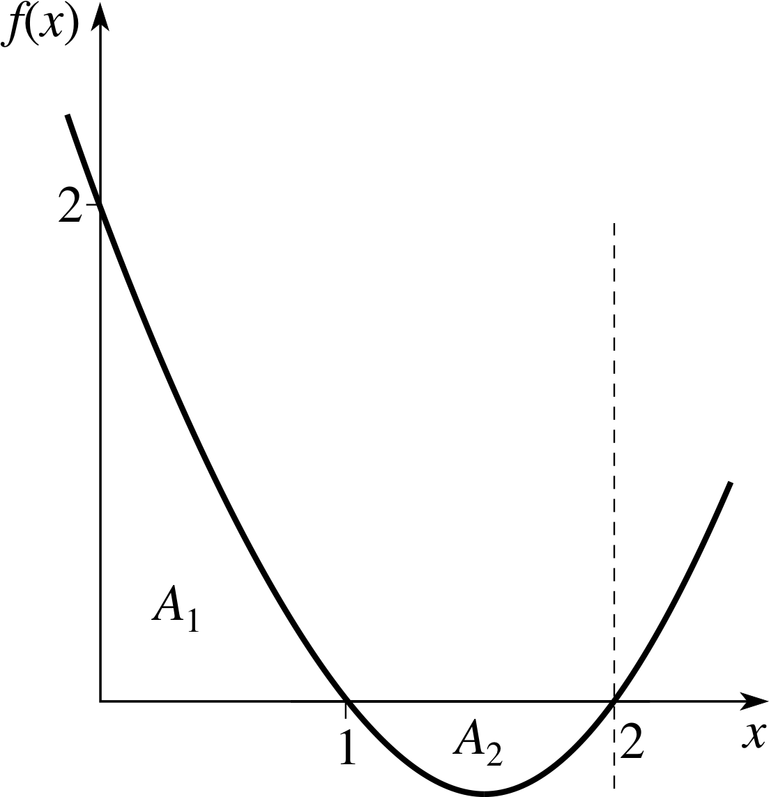
Figure 3 The function f (x) = x2 − 3x + 2.
Solution
As it is not immediately obvious whether f (x) = x2 − 3x + 2 changes sign between x = 0 and x = 2, we will start by sketching the function. This quadratic function factorizes: x2 − 3x + 2 = (x − 1)(x − 2). So the graph crosses the x–axis at x = 1 and at x = 2. When x = 0, f (x) = 2.
This gives us enough information to produce the sketch shown in Figure 3. We see that the region of interest is divided into two parts: one lying above the x–axis (labelled A1 in Figure 3) and another (A2) lying below. First we integrate f (x) between the limits x = 0 and x = 1 to find an integral I1 corresponding to the region A1
$I_1 = \Int_0^1(x^2 - 3x + 2)\,dx = \left[\frac13x^3 - \frac32x^2 + 2x\right]_0^1 = \frac13 - \frac32 + 2 = 0.833$
Now we integrate f (x) between x = 1 and x = 2 and find an integral corresponding to the region A2
$I_2 = \Int_1^2(x^2 - 3x + 2)\,dx = \left[\frac13x^3 - \frac32x^2 + 2x\right]_1^2 = \frac13(8-1) - \frac32(4-1) + 2(2-1) = -0.167$
i.e. a negative answer, because f (x) is always negative in this region. The magnitude of the area required is therefore
I1 + | I2 | = 0.833 + | −0.167 | = 0.833 + 0.167 = 1.000 i
In a question of this kind it is absolutely essential to be able to determine where the function changes sign; it will also help if you are able to sketch the graph of the function.
Question T1
Find the sum of the magnitudes of the areas enclosed by the graph of f (x) = ex − 2, the x–axis, and the lines x = 0 and x = loge 3. (You should start by sketching the graph.)
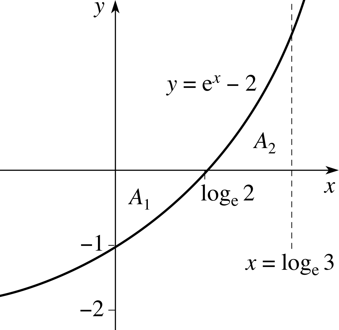
Figure 31 See Answer T1.
Answer T1
The graph of f (x) = ex − 2 is sketched in Figure 31; it crosses the x–axis where ex = 2, i.e. at x = loge 2. Since f (x) changes sign over the interval 0 ≤ x ≤ loge 3, we must evaluate the areas under the graph in two parts, and add their magnitudes to obtain the required answer. The area A1 is given by the integral of f (x) between 0 and loge 2:
$A_1 = \Int_0^{\loge 2}\left({\rm e}^x-2\right)\,dx = \left[{\rm e}^x-2x\right]_0^{\loge 2} = 2-2\loge 2-1 = -0.386$
(note that when we substituted in the limits, we used the fact that exp and loge are inverse functions, so that eloge2 = 2). Thus | A1 | = 0.386.
The area A2 is given by the integral of f (x) between loge 2 and loge 3:
$A_2 = \Int_{\loge 2}^{\loge 3}\left({\rm e}^x-2\right)\,dx = \left[{\rm e}^x-2x\right]_{\loge 2}^{\loge 3} = 3-2\loge 3-(2-2\loge 2) = 0.189$
So, the sum of the magnitudes of the areas is | A1 | + A1 = 0.386 + 0.189 = 0.575
We can summarize the previous discussion very neatly in terms of the modulus of f (x):
The magnitude_of_the_area_under_a_graphmagnitude of the area bounded by the graph of y = f (x) between the points x = a and x = b is given by the integral $\Int_a^b\lvert\,f(x)\rvert\,dx$. i
Since | f (x) | = f (x) when f (x) is positive, and | f (x) | = −f (x) when f (x) is negative, the modulus sign takes care of any changes in sign that f (x) may undergo in the region of integration. The integral $\Int_a^b\lvert\,f(x)\rvert\, dx$ is not in general equal to $\Int_a^bf(x)\,dx$; the two are only equal if f (x) ≥ 0 throughout the interval a ≤ x ≤ b.
Although this description is quite neat, in practice we rarely try to integrate | f (x) | directly, and usually we consider separately regions where the function is positive, and regions where the function is negative, as in Question T1.
The physical significance of the definite integral
So far, we have simply interpreted f (x) geometrically, as the height of the graph y = f (x), in which case $\Int_a^b\lvert\,f(x)\rvert\, dx$ is indeed just the magnitude of the area bounded by the graph of y = f (x), measured in whatever scale units are used on the graph’s axes. However, if f (x) represents some physical quantity, then the definite integral will of course have a different physical significance. Here are two examples.
Velocity–time graphs
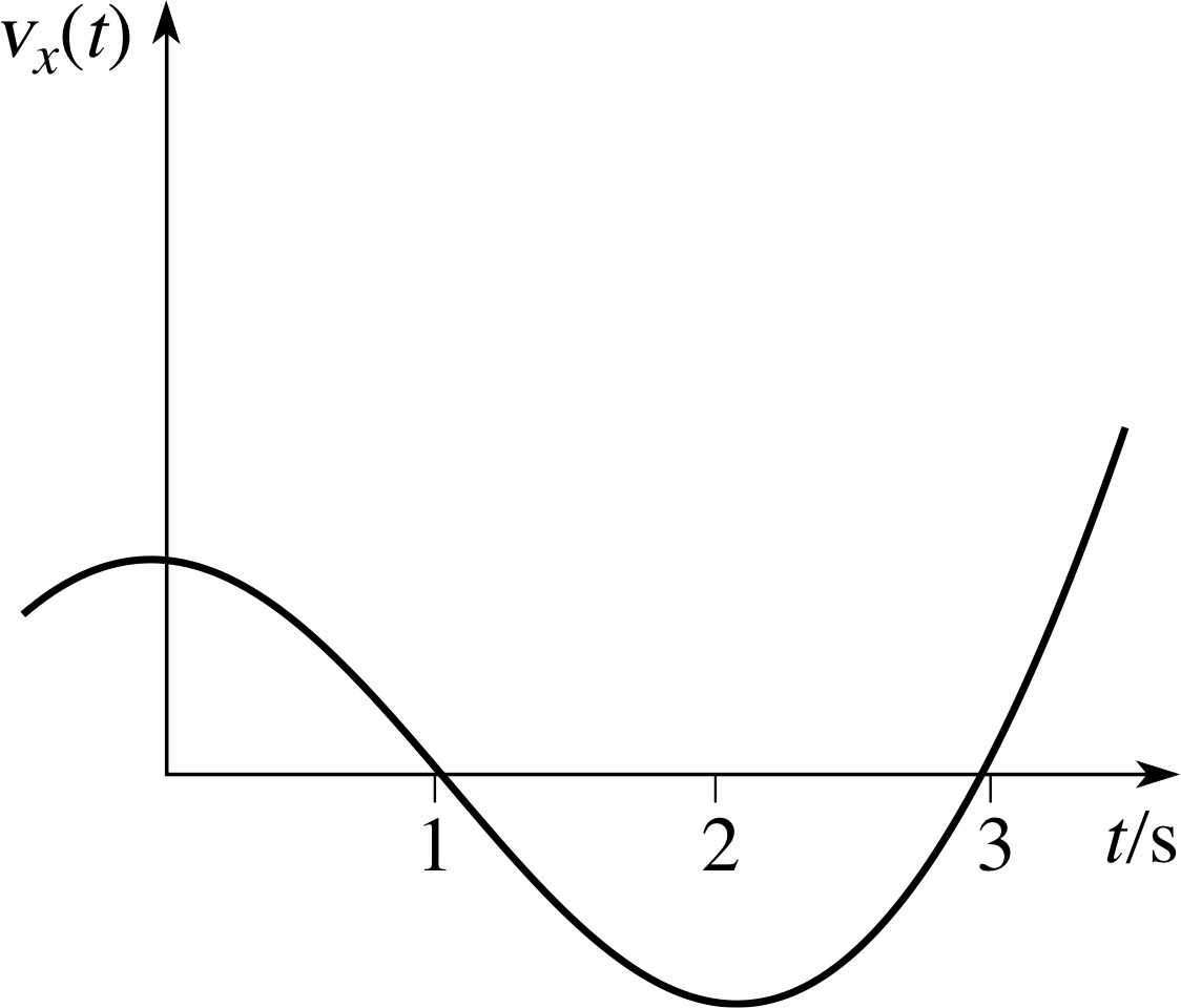
Figure 4 Velocity–time graph for an object moving along the x–axis.
Figure 4 shows a graph of the velocity, vx(t) of an object moving along the x–axis, against time t; note that vx(t) changes sign twice. If we want to know the displacement s x of the object from its initial position (at t = 0) after a given time T has elapsed, we can use the same reasoning that led from Equation 1 to Equation 2.
$\displaystyle A \approx \sum_{i=1}^n f(x_i)\,\Delta x_i$(Eqn 1)
$A = \Int_a^bf(x)\,dx$(Eqn 2)
We divide the time T into many short time intervals, each of duration ∆t. During any one of these time intervals, vx(t) is approximately constant, so the corresponding displacement is approximately equal to vx(t) ∆t; then the total displacement is approximately equal to the sum $\sum v_x(t)\,\Delta t$. In the limit as ∆t tends to zero, we find that the displacement is given by the integral $\Int_0^Tv_x(t)\,dt$, i.e. the area under the graph of vx(t) between t = 0 and t = T.
If, instead, we want to calculate the distance travelled by the object, we must recall that distance is the magnitude_of_a_real_quantitymagnitude of displacement. Thus the distance travelled in a short time interval ∆t is equal to | vx(t) | ∆t and, reasoning as before, we find that the distance travelled after time T is given by the integral $\Int_0^T\lvert\,v_x(t)\rvert\,dt$. So it is equal to the sum of the magnitudes of the areas enclosed by the graph of vx(t) and the t–axis, between t = 0 and t = T.
✦ An object is moving along the x–axis so that its velocity at time t is given by vx(t) = v0 sin(πt/T) m s−1, where v0 = 5 m s−1 and T = 1 s. What is its displacement after 2 s and what distance does it travel in the first 2 seconds?
✧ The displacement is
${\large\int}_0^{2\,{\rm s}}v_x(t)\,dt = {\Large\int}_0^{2\,{\rm s}}v_0\sin\left(\dfrac{\pi t}{T}\right)\,dt = \left[-\dfrac{v_0 T}{\pi}\cos\left(\dfrac{\pi t}{T}\right)\right]_0^{2\,{\rm s}} = -\dfrac{v_0 T}{\pi}\left[\cos(2\pi)-\cos(0)\right] = 0$
On the other hand, the distance travelled is
${\large\int}_0^{2\,{\rm s}}\left\vert\,v_x(t)\,\right\vert\,dt = {\Large\int}_0^{2\,{\rm s}}\left\vert\,v_0\sin\left(\dfrac{\pi t}{T}\right)\,\right\vert\,dt = \displaystyle v_0\int_0^{2\,{\rm s}}\left\vert\,\sin\left(\dfrac{\pi t}{T}\right)\,\right\vert\,dt$
$\phantom{{\large\int}_0^{2\,{\rm s}}\left\vert\,v_x(t)\,\right\vert\,dt \displaystyle }= v_0\left\{\int_0^{1\,{\rm s}}\sin\left(\dfrac{\pi t}{T}\right)\,dt + \int_{1\,{\rm s}}^{2\,{\rm s}}\left[-\sin\left(\dfrac{\pi t}{T}\right)\right]\,dt\right\}$ i
$\phantom{{\large\int}_0^{2\,{\rm s}}\left\vert\,v_x(t)\,\right\vert\,dt \displaystyle }= v_0 T\left\{\left[-\dfrac{1}{\pi}\cos\left(\dfrac{\pi t}{T}\right)\right]_0^{1\,{\rm s}} + \left[\dfrac{1}{\pi}\cos\left(\dfrac{\pi t}{T}\right)\right]_{1\,{\rm s}}^{2\,{\rm s}}\right\}$
$\phantom{{\large\int}_0^{2\,{\rm s}}\left\vert\,v_x(t)\,\right\vert\,dt \displaystyle }= \dfrac{v_0 T}{\pi}\left[(1+1)+(1+1)\right] = \dfrac{20}{\pi}\,{\rm m}$
Question T2
The graph shown in Figure 4 may be represented by the equation vx = at3 + bt2 + c, where a = 4 m s−4, b = −13 m s−3, c = 9 m s−1. Calculate (a) the displacement of the object, (b) the distance travelled by the object between t = 0 and t = 4 s.
Answer T2
(a) The displacement is given by the integral of vx(t) between t = 0 and t = 4 s:
$\Int_0^{4\,{\rm s}}(at^3+bt^2+c)\,dt = \left[\dfrac a4t^4+\dfrac b3t^3+ct\right]_0^{4\,{\rm s}} =14.667\,{\rm m}$
(b) The distance travelled, d say, is given by the integral of | vx(t) | between t = 0 and t = 4 s. As vx(t) changes sign at t = 1 s and t = 3 s, we must evaluate d in three stages. Between t = 0 and t = 1 s, vx(t) is positive. So | vx(t) | = vx(t) and the distance d1 travelled is:
$d_1 = \Int_0^{1\,{\rm s}}(at^3+bt^2+c)\,dt = \left[\dfrac a4t^4+\dfrac b3t^3+ct\right]_0^{1\,{\rm s}} = 5.667\,{\rm m}$
Between t = 1 s and t = 3 s, vx(t) is negative. So | vx(t) | = −vx(t) and the distance d2 travelled is
$d_2 = \Int_{1\,{\rm s}}^{3\,{\rm s}}(-at^3-bt^2-c)\,dt = \left[-\dfrac a4t^4-\dfrac b3t^3-ct\right]_{1\,{\rm s}}^{3\,{\rm s}} =14.667\,{\rm m}$
Between t = 3 s and t = 4 s, vx(t) is positive. So | vx(t) | = vx(t) and the distance d3 travelled is
$d_3 = \Int_{3\,{\rm s}}^{4\,{\rm s}}(at^3+bt^2+c)\,dt = \left[\dfrac a4t^4+\dfrac b3t^3+ct\right]_{3\,{\rm s}}^{4\,{\rm s}} = 23.667\,{\rm m}$
So, the total distance travelled is d = d1 + d2 + d3 = 44.001 m.
Work
Suppose that an object is moving along the x–axis under the influence of a constant force Fx in the x–direction. The work done by the force in moving the object from x = a to x = b is W = Fxsx where sx is the displacement of the object, which in this case is b − a.
If the force, Fx(x) say, varies with x, then we can divide the interval a ≤ x ≤ b into many much smaller subintervals, of width ∆x, in each of which Fx(x) is approximately constant. The work done in moving the object through the small subinterval between x and x + ∆x is approximately Fx(x) ∆x.
The total work done is approximately given by adding all these small amounts of work, so that
total work done $W \approx \sum F_x(x)\,\Delta x$
In the limit as ∆x decreases towards zero (and the number of subintervals increases) this approximation to W becomes increasingly accurate, and
$W = \Int_a^bF(x)\,dx$
It follows that we can interpret W to be the area under the graph of Fx(x) between x = a and x = b.
Question T3
A electric_chargepositively charged particle is fixed at the origin and a second positive charge moves away from it along the x–axis. The force acting on the second charge is A/x2 where the constant A = 7.3 × 10⁻²⁶ N m2. Calculate the work done on the charge as it moves from x = 0.1 m to x = 1.0 m.
Answer T3
The work done is $W = \INT_a^b\dfrac{A}{x^2}\,dx$, where a = 0.1 m and b = 1.0 m. Evaluating the integral gives
$W = \left[-\dfrac Ax\right]_a^b = \dfrac Aa - \dfrac Ab$
Putting in A = 7.3 × 10⁻²⁶ N m2, a = 0.1 m and b = 1.0 m gives
W = 7.3 × 10⁻²⁵ N m − 7.3 × 10⁻²⁶ N m = 6.6 × 10⁻²⁵ J
(Note that the work done is positive, as we would expect; the moving charge is being repelled by the stationary charge, and so its kinetic energy increases.)
2.2 Area between two graphs
Suppose that we want to find the area A enclosed by the graphs of the two functions f (x) and g (x) shown in Figure 5. Proceeding as before, we divide the region up into thin slices, each of thickness ∆x, then approximate each slice by a thin rectangle. The height of the rectangle shown in Figure 5 is (f (x) − g (x)), and so its area is (f (x) − g (x)) ∆x. We now sum the areas of all the rectangles, and let ∆x tend to zero, so that in the limit the sum becomes an integral and we have
$A = \Int_a^b\left[\,f(x) - g(x)\right]\,dx$(3)
where a and b are the x–coordinates of the points of intersection of the two graphs. Notice that f (x) ≥ g (x) in the interval a ≤ x ≤ b, which ensures that f (x) − g (x) is positive, and therefore A is also positive.
✦ Suppose f (x) = −x2 + 4x − 2 and g (x) = x2 − 4x + 4. The graphs of these functions intersect at x = 1 and x = 3. Use Equation 3 to find the area A enclosed by these graphs.
✧ f (x) − g (x) = −2x2 + 8x − 6 = 2 (x − 1)(3 − x) ≥ 0 if 1 ≤ x ≤ 3.
So$A = {\large\int}_1^3(2x^2 + 8x - 6)\,dx = \left[-\frac23x^3 + 4x^2 - 6x\right]_1^3 = -\frac23(27-1)+4(9-1)-6(3-1) = 2.667$
It is quite possible to find such an area without drawing the graphs (as the above exercise shows), but if you are asked to calculate the area between the graphs of f (x) and g (x), you will find it much easier if you begin by sketching the two graphs on the same axes, and, of course, finding the points of intersection (which you need in order to be able to put in the correct limits in Equation 3).
The following example shows you how to proceed.
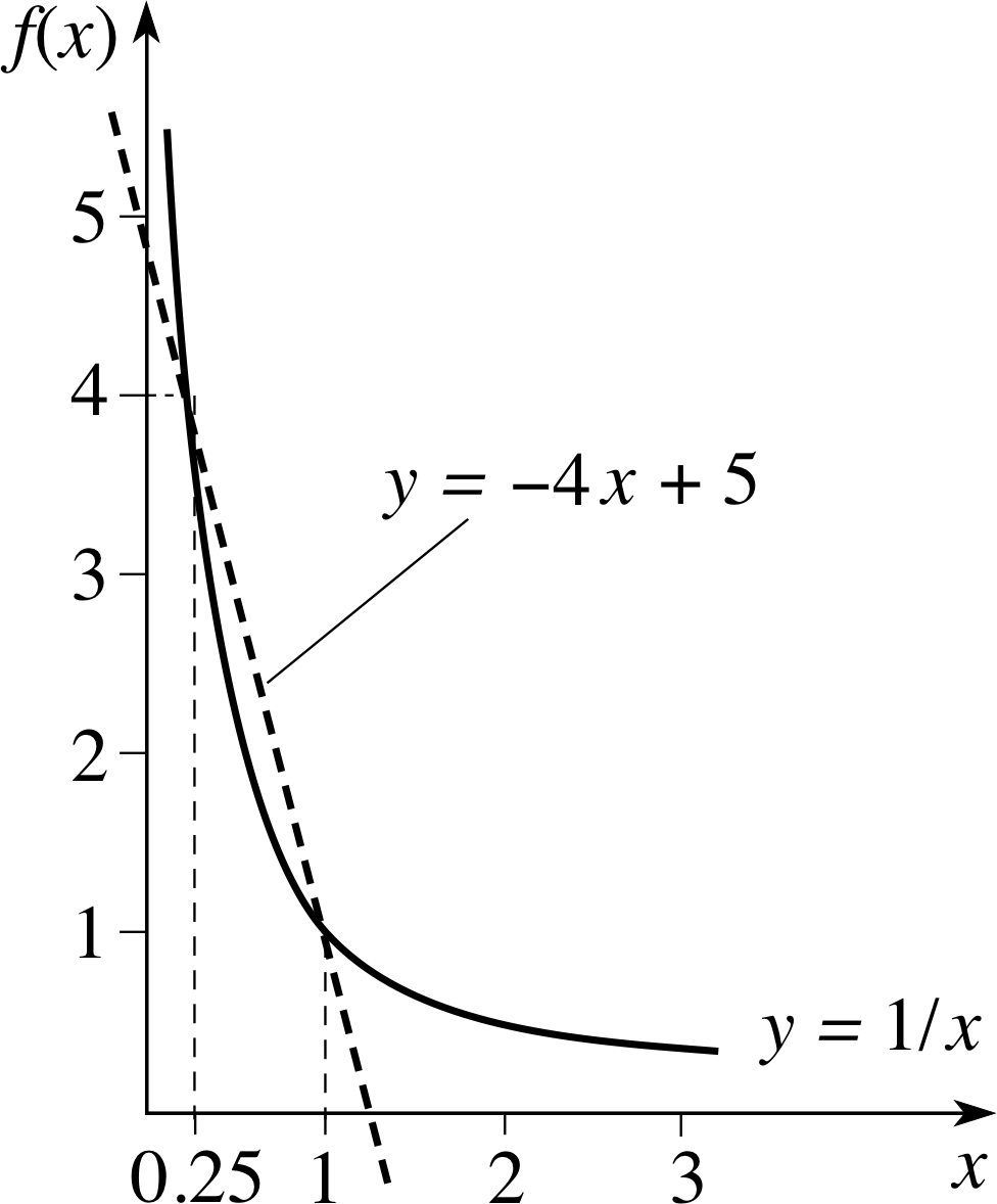
Figure 6 See Example 2.
Example 2
Find the area between the line y = f (x) = −4x + 5 and the graph of g (x) = 1/x.
Solution
The two graphs intersect where −4 x + 5 = 1/x. Rearranging this equation gives us a quadratic equation to solve for x namely 4x2 − 5x + 1 = 0, which factorizes to give (x − 1)(4x − 1) = 0. So we see that the roots of this equation are x = 1 and x = 1/4.
We can now sketch the area enclosed by the two graphs, showing the points of intersection (see Figure 6).
We now evaluate the area, using Equation 3:
$A =\Int_{1/4}^1(-4x + 5 - 1/x)\,dx = \left[-2x^2 + 5x - \loge x\right]_{1/4}^1$
$\phantom{A }= -2(1-1/16) + 5(1-1/4) - \loge 1 + \loge 1/4 = 0.4887$
Question T4
Find the area between the graphs of $f(x) = 8\sqrt{x\os}$ and g (x) = x2. (Start by sketching the two graphs.)
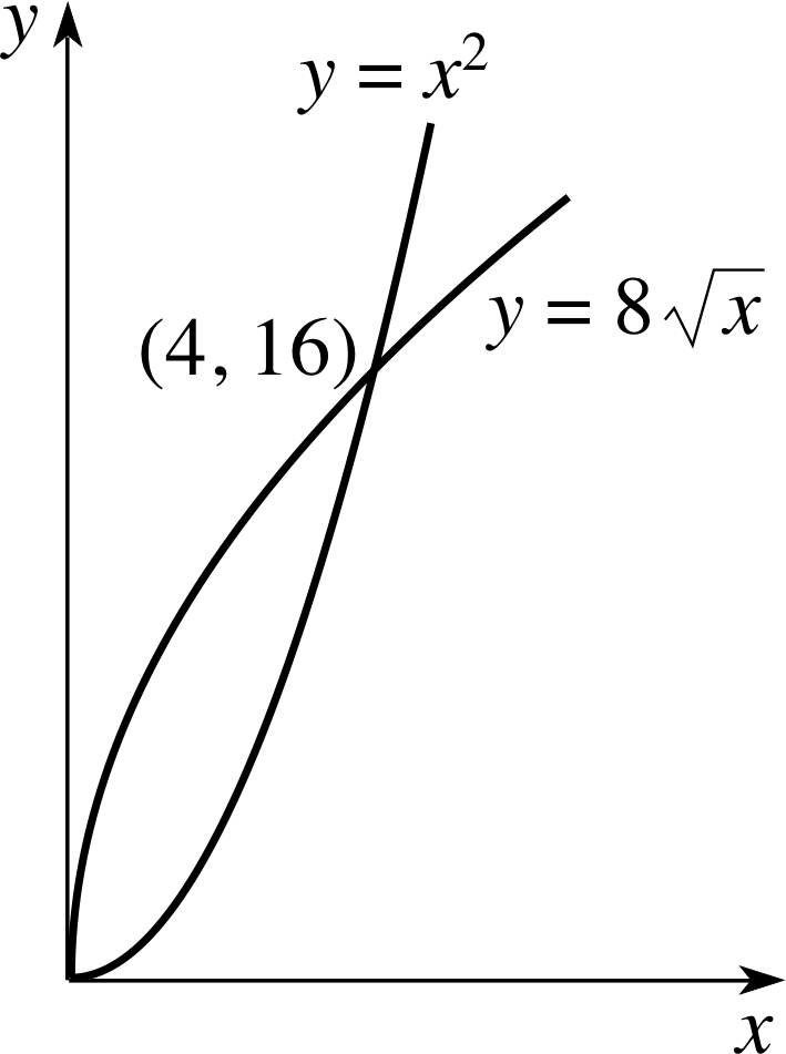
Figure 32 See Answer T4.
Answer T4
The graphs of $f(x) = 8\sqrt{x\os}$ and g (x) = x2 intersect where $8\sqrt{x\os} = x^2$, i.e. at x = 0 and where x3/2 = 8, or x = 4. They are shown in Figure 32. The area between the graphs is given by Equation 3,
$A = \Int_a^b\left[\,f(x) - g(x)\right]\,dx$(3)
(with a = 0 and b = 4):
$A= \Int_0^8\left(8\sqrt{x\os}-x^2\right)\,dx = \left[\frac{16}{3}x^{3/2}-\frac13x^3\right]_0^8 = 21.333$
In all the examples so far, the functions f (x) and g (x) have been chosen so that the graph of f (x) lies above the graph of g (x). This ensures that the integrand in Equation 3,
$A = \Int_a^b\left[\,f(x) - g(x)\right]\,dx$(Eqn 3)
is positive, so that we obtain a positive answer for A. If we had chosen our two graphs the other way round, then the height of the rectangle in Figure 5 would have been equal to (g (x) − f (x)), and it is this function that we would have integrated. Thus, wherever f (x) > g (x), we integrate (f (x) − g (x)), to obtain the area; but in the case that g (x) > f (x), we integrate (g (x) − f (x)). In both these cases, we can write down the area of the region – known as the area_between_two_graphsarea between the graphs of f (x) and g (x) – as
$A =\Int_a^b\left\lvert\;f(x) - g(x)\,\right\rvert\,dx$(4)
It is important to use Equation 4 (not Equation 3) if the two graphs intersect more than twice, so that (f (x) − g (x)) is sometimes positive and sometimes negative, as in the next example. i
Example 3
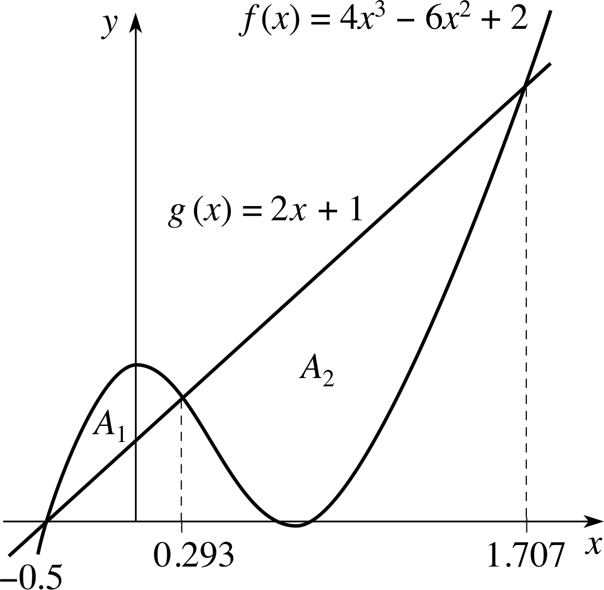
Figure 7 See Example 3. Note that the horizontal and vertical scales on the graph have been made different for convenience of drawing.
Figure 7 shows the graph of f (x) = 4x3 − 6x2 + 2 and the line g (x) = 2x + 1. They have three points of intersection, at x = −1/2, $x = 1 - 1/\sqrt{2\os} = 0.293$ and $x = 1 + 1/\sqrt{2\os} = 1.707$. i
Find the total area enclosed by the two graphs.
Solution
Over the region −1/2 < x < 0.293, f (x) is greater than g (x). Thus the area labelled A1 in Figure 7 is given by integrating (f (x) − g (x)) = 4x3 − 6x2 − 2x + 1 from x = −1/2 to x = 0.293:
$A_1 = \Int_{-0.5}^{0.293}(4x^3 - 6x^2 - 2x + 1)\,dx = \left[x^4 - 2x^3 - x^2 + x\right]_{-0.5}^{0.293}$
$\phantom{A_1 } = 0.164 - (-0.438) = 0.602$
Over the region 0.293 < x < 1.707, f (x) is less than g (x). Thus the area labelled A2 in Figure 7 is given by integrating | (f (x) − g (x)) | = g (x) − f (x) = −4x3 + 6x2 + 2x − 1 from x = 0.293 to x = 1.707.
$A_2 = \Int_{0.293}^{1.707}(-4x^3 + 6x^2 + 2x - 1)\,dx = -\left[x^4 - 2x^3 - x^2 + x\right]_{0.293}^{1.707}$
$\phantom{A_2 } = 2.664 - (-0.164) = 2.828$
So the total area is 0.602 + 2.828 = 3.430.
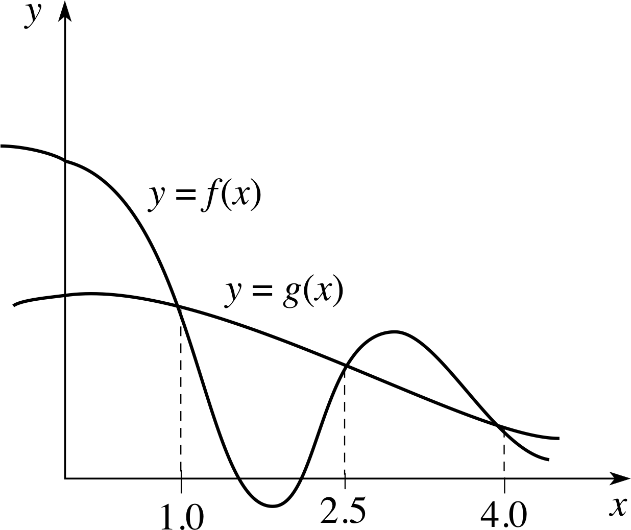
Figure 8 An area enclosed by two graphs between x = 1.0 and x = 4.0.
✦ Figure 8 shows the graphs of two functions f (x) and g (x); their points of intersection are given as x = 1.0, x = 2.5 and x = 4.0. Write down the two integrals whose sum gives the total area enclosed by the graphs.
✧ Since f (x) < g (x) for 1.0 < x < 2.5, and f (x) > g (x) for 2.5 < x < 4.0, the two integrals are
${\large\int}_{1.0}^{2.5}[g(x) - f(x)]\,dx$ and ${\large\int}_{2.5}^{4.0}[f(x) - g(x)]\,dx$
The area of a circle
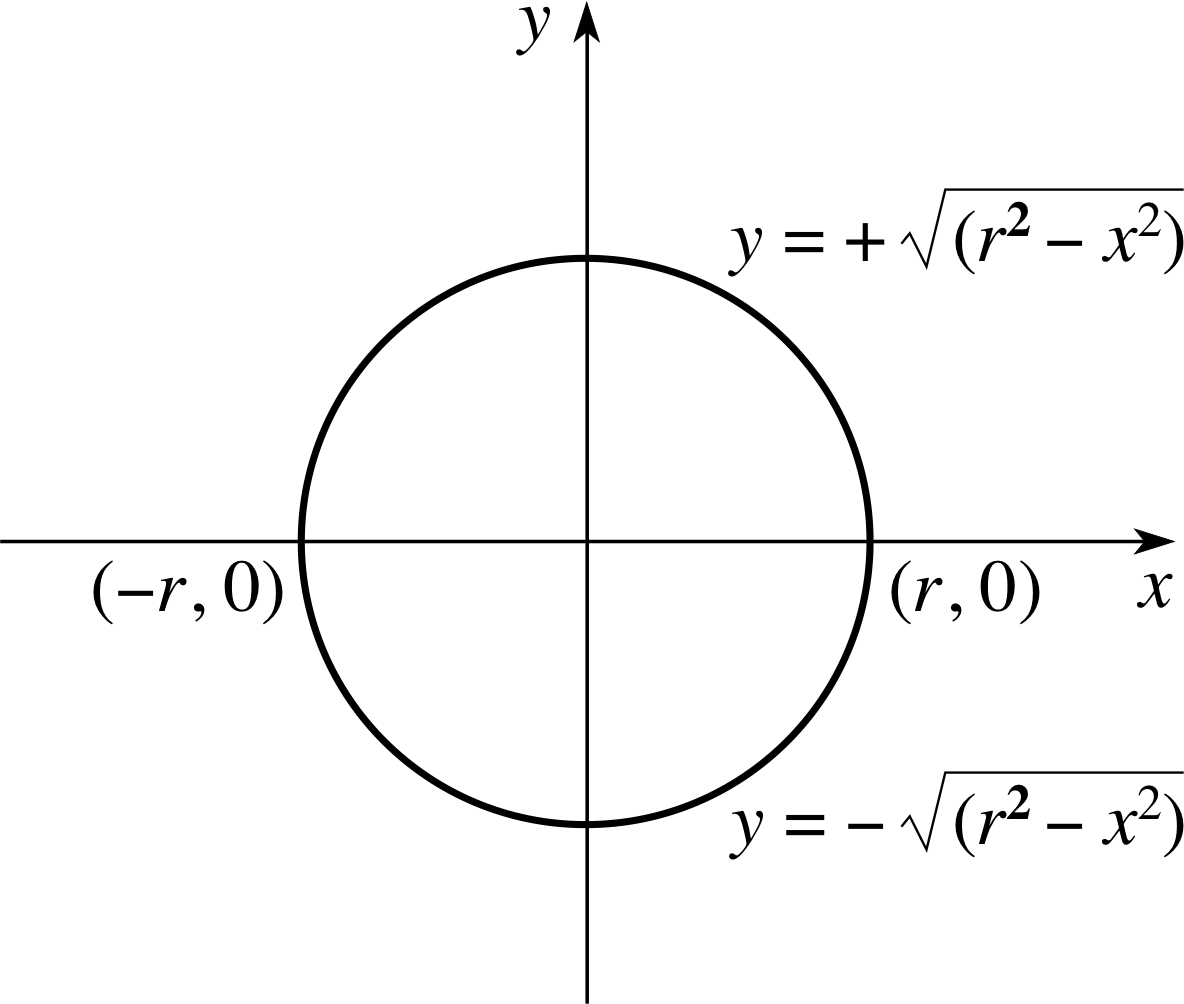
Figure 9 The circle x2 + y2 = r2.
Finally in this subsection, it is worth noting that we can use Equation 4,
$A =\Int_a^b\lvert\,f(x) - g(x)\rvert\,dx$(Eqn 4)
to find the areas of shapes such as circles and ellipses. For example, let us use it to prove that the area of a circle of radius r is πr2. The equation of a circle of radius r centred on the origin is x2 + y2 = r2; so, for a given value of x (less than r), y can take the two values $+\sqrt{r^2-x^2}$ and $-\sqrt{r^2-x^2}$. Thus we can regard the region inside the circle as the area enclosed by the graphs of the two functions $f(x) = +\sqrt{r^2-x^2}$ and $g(x) = -\sqrt{r^2-x^2}$ (see Figure 9). The points of intersection of these two graphs are x = − r and x = + r. So Equation 4 gives, for the area A of the circle,
$A = \Int_{-r}^r\left[\sqrt{r^2-x^2}-\left(-\sqrt{r^2-x^2}\right)\right]\,dx = 2\Int_{-r}^r(\sqrt{r^2-x^2})\,dx$
The definite integral can be evaluated by making the substitution x = rsin u. Then $\sqrt{r^2-x^2} = \sqrt{r^2 (1 - \sin^2u)} = r\cos u$, and dx = r cos u du.
When x = r, sin(u) = 1, so u = π/2, and when x = −r, u = −π/2; thus the new limits of integration are π/2 and −π/2. So the integral becomes
$A = 2r^2 \Int_{-\pi/2}^{\pi/2}\cos^2 u\,du$
We can evaluate this integral by means of the trigonometric identity 2 cos2u = 1 + cos(2u); substituting this into the integral, we find
$\displaystyle A = 2r^2 \int_{-/pi2/}^{\pi/2}\cos^2 u\,du = 2r^2\int_{-/pi2/}^{\pi/2}\dfrac12\{1+\cos(2u)\}\,du = r^2\left[u+\dfrac12\sin(2u)\right]_{-/pi2}^{\pi/2}$
$\phantom{A }= r^2\left[\dfrac{\pi}{2}+\dfrac12\sin(\pi) - \left(-\dfrac{\pi}{2}+\dfrac12\sin(-\pi)\right)\right] = \pi r^2$
Question T5
Find the area enclosed by the ellipse x2/16 + y2/9 = 1.
Answer T5
We first rearrange the equation of the ellipse as y2 = 9 (1 − x2/16). We see from this that we can regard the ellipse (sketched in Figure 33) as being bounded by the graphs of the two functions $f(x) = 3\sqrt{1 - x^2/16}$ and $g(x) = -3\sqrt{1 - x^2/16}$, which intersect at x = −4 and x = 4. So the area of the ellipse is given by
$\displaystyle A = \int_{-4}^4\left\{\left(3\sqrt{1-x^2/16}\right)-\left(-3\sqrt{1-x^2/16}\right)\right\}\,dx = 6 \int_{-4}^4\sqrt{\left(1-x^2/16\right)}\,dx$
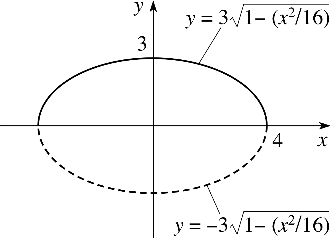
Figure 33 See Answer T5.
This integral can be evaluated using the substitution x = 4 sin u; then the integrand becomes cos u and dx = 4 cos u du. The new limits of integration are u = −π/2 (when x = −4 and sin u = −1) and u = π/2 (when x = 4 and sin u = 1).
So,$A = 24\Int_{-\pi/2}^{\pi/2}\cos^2u\,du$
We now use the trigonometric identity 2 cos2(u) = 1 + cos 2u; which gives:
$A = 12\Int_{-\pi/2}^{\pi/2}(1+\cos 2u)\,du = 12\left[u+\frac12\sin 2u\right]_{-\pi/2}^{\pi/2} = 12\pi$
3 Solids of revolution
3.1 Volume of revolution
Suppose that we want to find the volume of a cone, of height h and base radius r. Such a cone is shown in Figure 10; we have drawn it so that its vertex is at the origin and its axis of symmetry lies along the x–axis. To find the volume we can approximate the cone by a set of thin discs, each of thickness ∆x. One of these discs, D, is shown in Figure 10. The centre of the disc D has coordinates (x, 0). We calculate the volume of each disc, and then obtain an estimate for the volume of the cone by adding these volumes. We then allow ∆x to tend to zero, and in the limit the sum becomes a definite integral between the limits 0 and h, which gives the exact value of the volume of the cone. In order to be able to evaluate this integral, we must, of course, obtain an expression for the volume of a typical disc in terms of x.
To calculate the volume of a typical disc D, we need first to know its radius. This is equal to the y–coordinate of the point A, and to express this in terms of x, we need to find the equation of the line OP in Figure 10. This line passes through the origin and the point (h, r); its gradient is r/h and its intercept is zero. So the equation of the line is y = rx/h. Consequently, the radius of the disc D is rx/h.
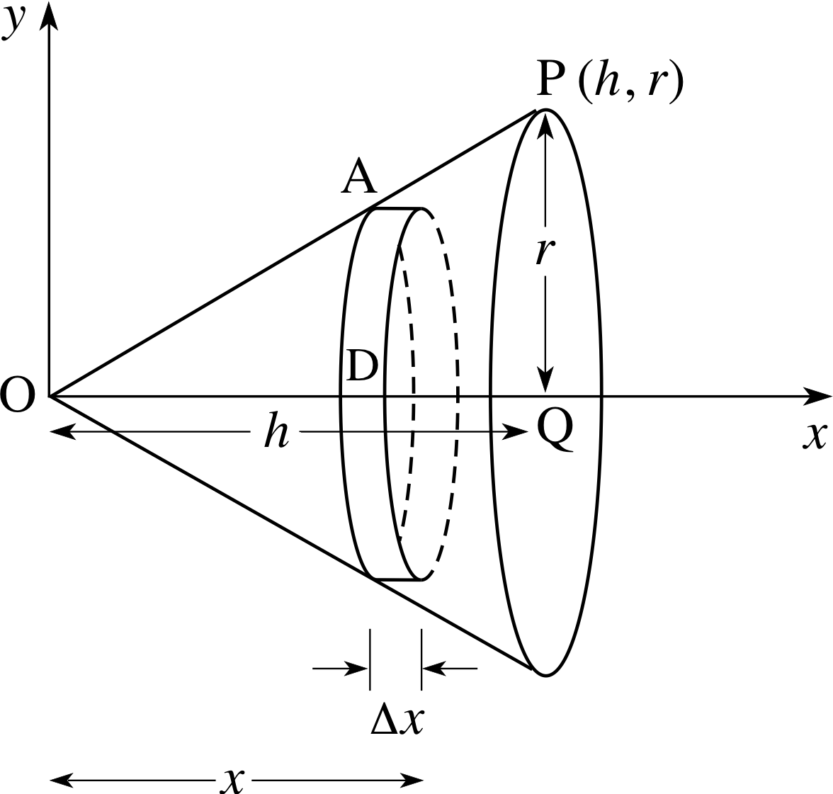
Figure 10 A cone of height h and
Hence
cross-sectional area of $D = \pi\left(\dfrac rh\right)^2$
and
volume of D = area × thickness = $D = \pi\left(\dfrac rh\right)^2x^2\Delta x$
Hence the volume V of the cone is given by the integral
$V = \pi\left(\dfrac rh\right)^2\Int_0^hx^2\,dx = \pi\left(\dfrac rh\right)^2\left[\dfrac13x^3\right]_0^h = \frac13\pi r^2h$
an expression that you have probably seen before.
We will show shortly that we can generalize this strategy to find the volume of any solid which can be regarded, to a good approximation, as a series of discs all centred on the x–axis. But we first introduce some terminology.
Look at Figure 10; imagine rotating the triangle OPQ (which lies in the (x, y) plane) about the x–axis. As you do so, the line OP will sweep out the surface of the cone. We can say, therefore, that the cone is generated by rotating the area OPQ about the x–axis. This is an example of a solid of revolution a solid which can be obtained by rotating the area under a graph (or part of a graph) about some axis. The volume of a solid of revolution is known as a volume of revolution.
✦ Describe the solid of revolution obtained by rotating the area under the line y = 3 between x = 2 and x = 6 about the x–axis.
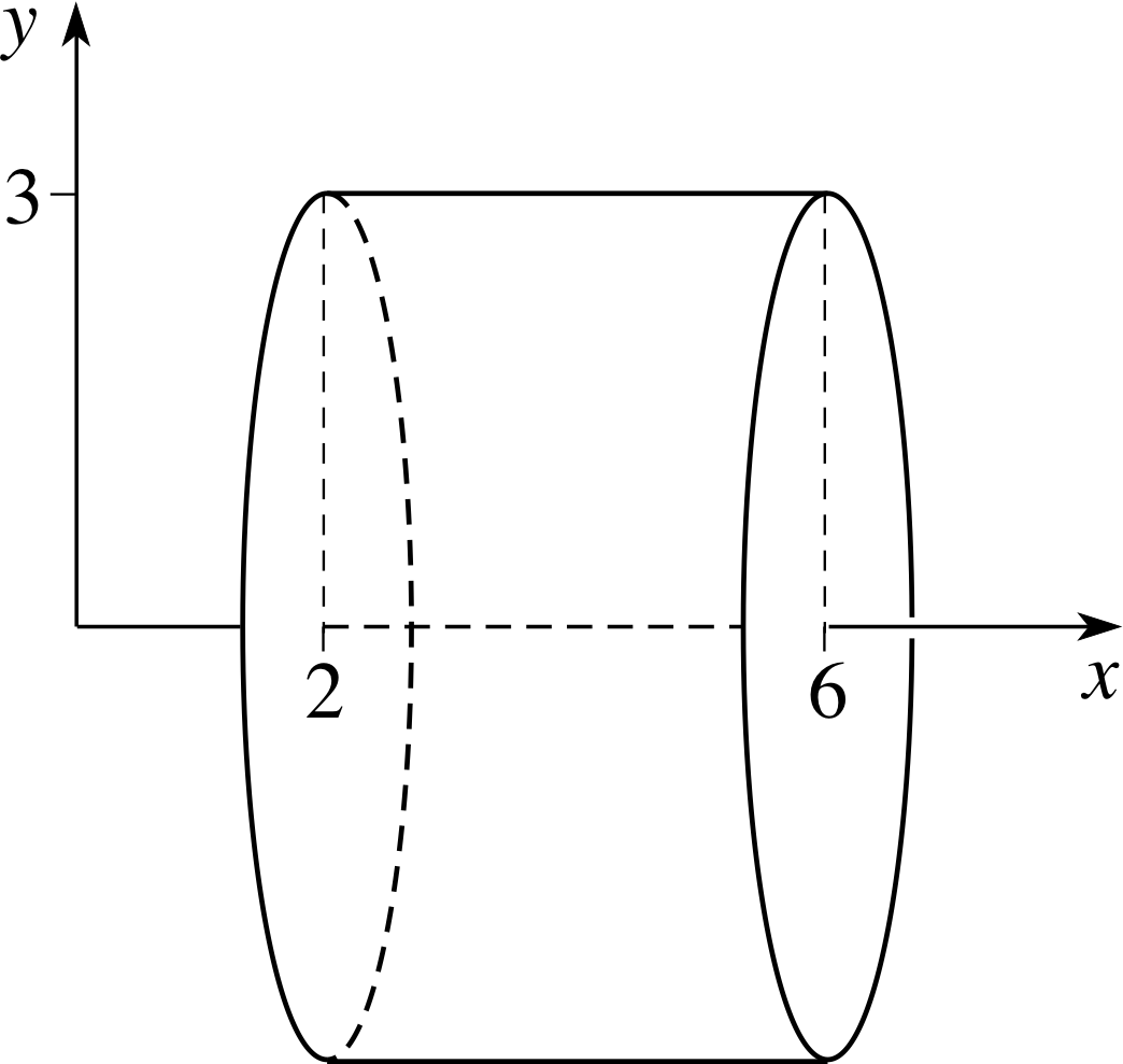
Figure 11 The solid obtained by rotating the area under the line y = 3 between x = 2 and x = 6 about the x–axis.
✧ This solid is a cylinder, of radius 3 and height 4 (see Figure 11).
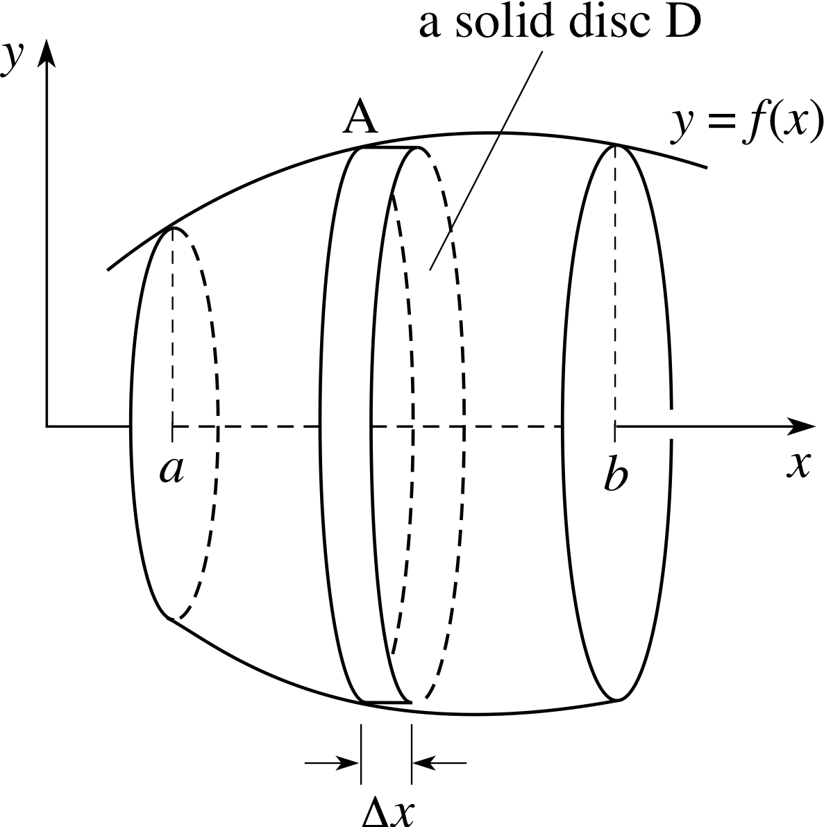
Figure 12 Solid of revolution obtained by rotating the area under the graph of f (x) about the x–axis.
Figure 12 shows an arbitrary solid of revolution, obtained by rotating the area under the graph of the function f (x) between the points x = a and x = b about the x–axis. As we did with the cone, we can approximate this volume by a set of thin discs of thickness ∆x; we show one such disc, D, in Figure 12. The radius of D is equal to the y–coordinate of the point A; that is, it is equal to f (x).
So the cross–sectional area of D is π [f (x)]2, and its volume is π [f (x)]2 ∆x.
Summing over the volumes of all the discs, and allowing ∆x to tend to zero, we obtain a definite integral for the volume V of the solid of revolution:
$V = \pi\Int_a^b\left[\,f(x)\right]^2\,dx$(5)
Example 4
The solid of revolution obtained by rotating the semicircle $f(x) = \sqrt{r^2 - x^2}$ about the x–axis is a sphere of radius r. Use Equation 5 to show that the volume of a sphere of radius r is $\frac43\pi r^3$.
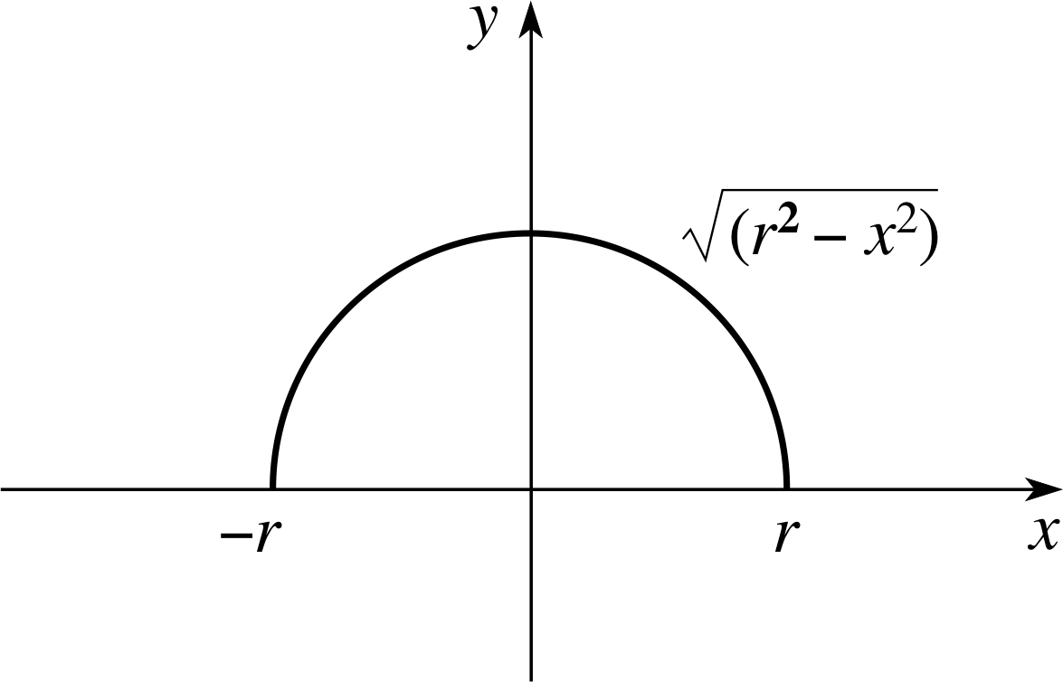
Figure 13 See Example 4.
Solution
We first sketch the semicircle (see Figure 13); this shows us y that the limits of integration are x = −r and x = +r. Then we substitute these limits and $f(x) = \sqrt{r^2 - x^2}$ into Equation 5 to obtain
$V = \pi\Int_{-r}^r(r^2 - x^2)\,dx$
Evaluating the integral gives us
$V = \pi\left[r^2x-\frac13x^3\right]_{-r}^r = \pi\left\{\frac23r^3-\left(-\frac23r^3\right)\right\} = \frac43\pi r^3$
Question T6
Find the volume of revolution obtained by rotating the area under the graph of f (x) = 3x2 between x = 1 and x = 3 about the x–axis.
Answer T6
To find this volume V of revolution, we use Equation 5,
$V = \pi\Int_a^b\left[\,f(x)\right]^2\,dx$(5)
with f (x) = 3/x2, a = 1 and b = 3. Then:
$V = \pi\Int_1^3x^4\,dx = \pi\left[-\dfrac{3}{x^3}\right]_1^3 = \pi(-0.111+3) = 9.076$
3.2 Surface of revolution
Figure 10 A cone of height h and base radius r.
Suppose now that we want to find, not the volume but the surface area of the cone shown in Figure 10. By now, you may be thinking that you know what is coming. Perhaps what we must do is to approximate the cone by a set of thin discs (just as we did to calculate its volume), work out the surface area of a typical disc, add up all these surface areas, and let the thickness of the discs tend to zero, to obtain an integral giving the surface area of the cone. This process does NOT work, and an example should convince you that this is the case.
The disc D in Figure 10 has radius rx/h, its circumference is 2πrx/h, and so its surface area (= circumference × thickness) is 2πrx/h ∆x. Thus the integral giving the total surface area of the discs as their thickness tends to zero is
$2\pi\dfrac rh\Int_0^hx\,dx = 2\pi\dfrac rh\left[\dfrac12x^2\right]_0^h = \pi rh$(6)
However, Equation 6 does not give the correct answer for the surface area of the cone, as we can easily verify!
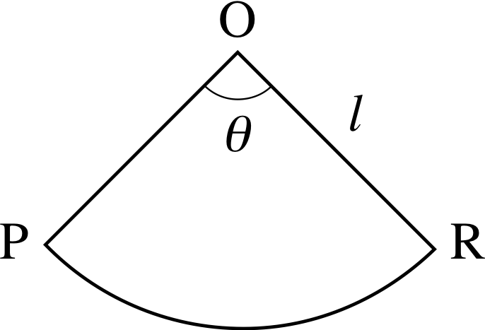
Figure 14 An unrolled cone.
We have another way of finding this surface area: we can imagine cutting the cone along a straight line running from its base to its vertex and spreading the cone out flat. This gives us the sector of a circle shown in Figure 14; the radius of the circle is equal to the slant height l of the cone (i.e. the length of the line OP in Figures 10 and 14), and the length of the arc PR is equal to the circumference of the base of the cone, 2πr. (If you do not believe that this is the figure obtained, try doing th eexperiment in reverse. Cut out a sector of a circle; you will find that you can roll it up into a cone.)
The surface area of the cone is equal to the area of the sector shown in Figure 14. This sector is a fraction θ/2π of the complete circle of radius l, where θ is the angle $\rm{P\hat{O}R}$ (measured in radians).
So its area must be equal to (θ/2π) × the area of this circle (πl2), i.e. to $\frac12\theta l^2$.
The angle θ is equal to the length of the arc PR divided by the radius l of the circle, θ = 2πr/l, so we find
surface area S of cone = $\dfrac12\left(\dfrac{2\pi r}{l}\right)l^2 = \pi rl$(7)
– NOT the same as the result obtained in Equation 6.
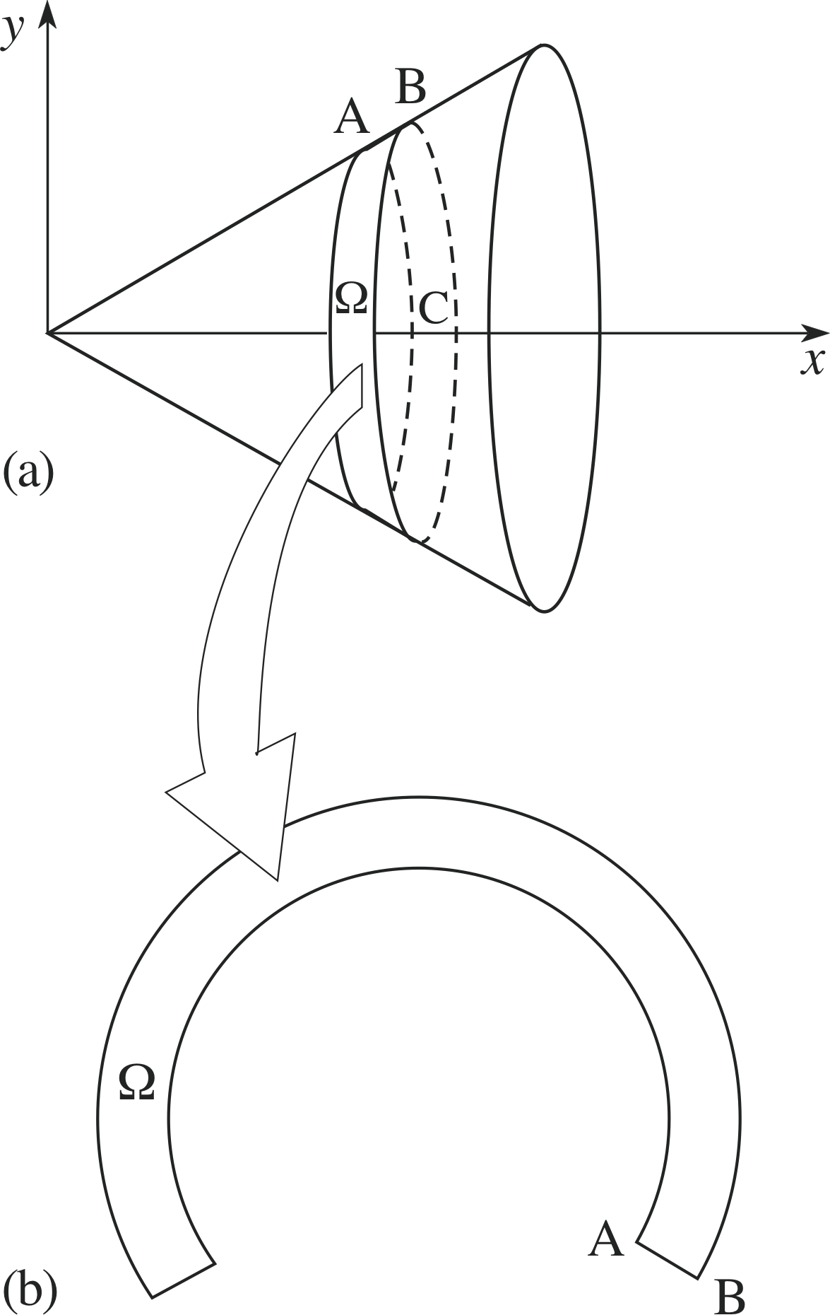
Figure 15 (a) A slice of a cone. (b) The unwrapped slice Ω.
The reason why Equation 6 gives the wrong answer is simply that, while the volume of a thin slice of the cone is well approximated by the volume of a thin disc of the same thickness and with radius equal to the average radius of the slice, the surface area of such a slice is not equal, even approximately, to the surface area of the corresponding disc. However, we can arrive at an integral giving the surface area of the cone if we consider carefully what the surface area of a thin slice of it actually is.
Figure 15a shows such a slice Ω, whose thickness (equal to the length AB) we will call ∆s. We can think of this slice as being generated by rotating the line segment AB about the x–axis; in which case we see that the point B travels a total distance equal to 2π × BC. So if we imagine cutting the slice along AB, and laying it flat, we will obtain the shape shown in Figure 15b part of a ring. The area of this region is, to a good approximation, given by the product of its thickness ∆s and the length of the outer arc bounding it, 2π × BC:
area of slice Ω = 2π × BC × ∆s(8)
Before we can use Equation 8 to give us an integral equal to the surface area of the cone, we must express all quantities in it in terms of x. The length BC is equal to the y–coordinate of the point B, which is equal to rx/h. We now need to relate ∆s to ∆x, and this can be done using Pythagoras’s theorem.
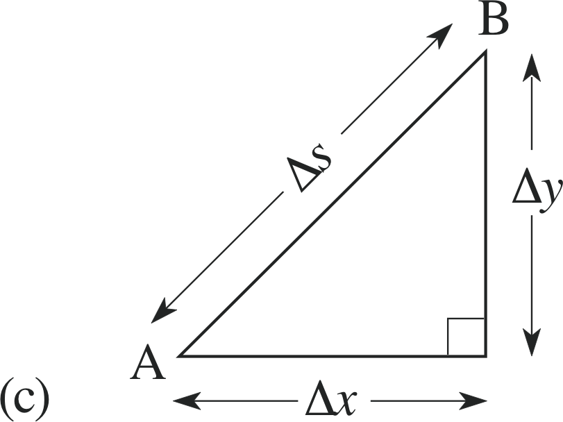
Figure 15 (c) The length ∆s in terms of ∆x and ∆y.
From Figure 15c, we see that (∆s)2 = (∆x)2 + (∆y)2 = (∆x)2 (1 + (∆y)2/(∆x)2)
i.e.$\Delta s = \Delta x\sqrt{1+(\Delta y)^2/(\Delta x)^2}$
The ratio ∆y/∆x is simply equal to the gradient of the line OP, which is r/h. So we have
$\Delta s = \Delta x\sqrt{1 + \dfrac{r^2}{h^2}}$
and substituting this, and BC = rx/h in Equation 8, we find
area of the slice Ω = $2\pi~~\underbrace{\dfrac rhx}_{\color{purple}{\large{\rm BC}}}~~\underbrace{\left(\sqrt{1 + \dfrac{r^2}{h^2}}\right)\Delta x}_{\color{purple}{\large{\Delta x}}}$
We now add up all such areas, allow the thickness of the slices to tend to zero, and so obtain a definite integral for the surface area S of the cone:
$\displaystyle S = 2\pi\int_0^h\left(\dfrac rhx\sqrt{1 + \dfrac{r^2}{h^2}}\right)\,dx = 2\pi\underbrace{\dfrac rh\sqrt{1 + \dfrac{r^2}{h^2}}}_{\color{purple}{\large{\substack{\text{everything here}\\[2pt]\text{is constant}}}}}{\small\int}_0^hx\,dx$
✦ Evaluate the above integral, to get an expression for S.
✧
$S = 2\pi\dfrac rh\sqrt{1+\dfrac{r^2}{h^2}}\left[\dfrac12x^2\right]_0^h = \pi rh\sqrt{1+\dfrac{r^2}{h^2}}$(9)
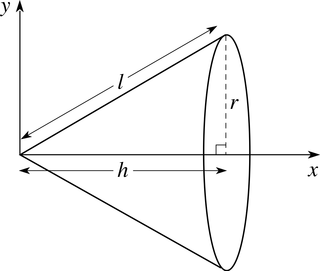
Figure 16 Relation between slant height l, height h and radius r of a cone.
The answer you have found does not yet look quite the same as the answer obtained in Equation 7, which was πrl. However, it is not hard to show that it is in fact the same. Figure 16 shows that the slant height l, the height h and the radius r of the cone are related by Pythagoras’s theorem: l2 = h2 + r2, which can be rearranged to give $l = h\sqrt{ 1 + r^2/h^2}$. So the right–hand sides of Equation 9,
$S = 2\pi\dfrac rh\sqrt{1+\dfrac{r^2}{h^2}}\left[\dfrac12x^2\right]_0^h = \pi rh\sqrt{1+\dfrac{r^2}{h^2}}$(Eqn 9)
and Equation 7,
surface area S of cone = $\dfrac12\left(\dfrac{2\pi r}{l}\right)l^2 = \pi rl$(Eqn 7)
are identical.
Now that we have seen how to write the surface area of a cone as an integral, we can generalize the method to find the area of any surface of revolution that is, any surface produced by rotating a graph about an axis.
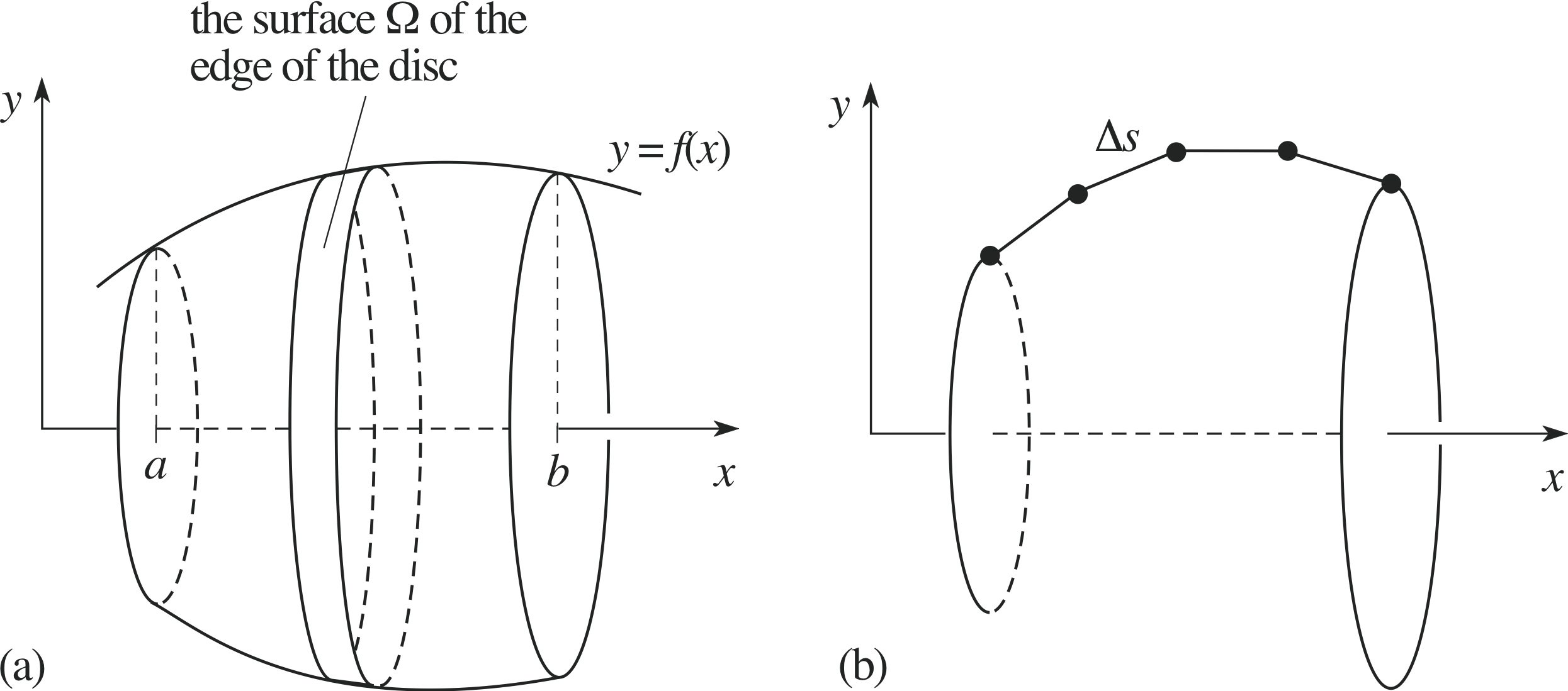
Figure 17 (a) The surface of revolution produced by the graph of f (x) between the points x = a and x = b. (b) An approximation to the graph of f (x).
Figure 17a shows the graph of the function f (x) and its surface of revolution between the points x = a and x = b. To find the surface of revolution S, we approximate the graph by a set of line segments of equal length ∆s, as shown in Figure 17b. When one of these is rotated about the x–axis, it generates a surface Ω whose surface area is approximately equal to that of a slice of the solid of revolution. The area of the surface Ω is approximately equal to its thickness ∆s multiplied by the distance travelled by one end of the line segment as it is rotated about the x–axis, 2π f (x). So we have
area of Ω ≈ 2π f (x) ∆s(10)
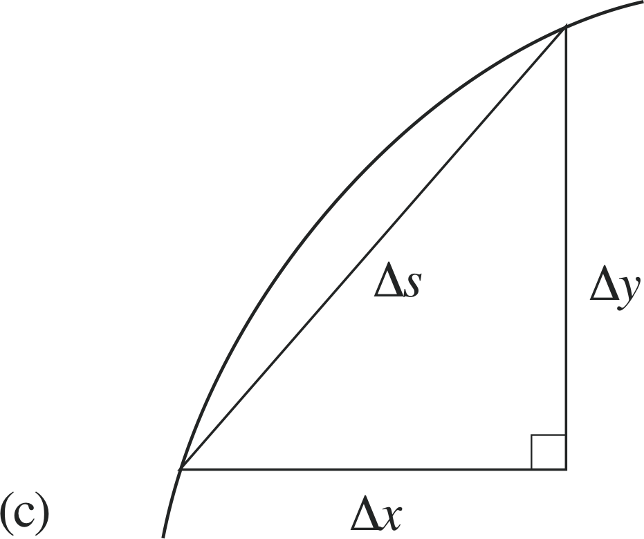
Figure 17 (c) Approximation for the length ∆s in terms of ∆x and ∆y.
Figure 17c shows that in this general case, we have the approximate relation
$\Delta s \approx \sqrt{(\Delta x)^2 + (\Delta y)^2} = \Delta x \sqrt{1+(\Delta y/\Delta x)^2}$(11)
This approximation will become better as ∆x and ∆s get smaller and smaller. We can also write
$\Delta y \approx \dfrac{dy}{dx}\Delta x$ i.e. ∆y ≈ f ′ (x) ∆x(12)
and again, this approximation will improve as ∆x tends to zero. Substituting Equations 11 and 12 into Equation 10 gives
area of the thin strip Ω ≈ $\underbrace{2\pi\,f(x)}_{\color{purple}{\large\substack{\text{length of}\\[2pt]\text{the strip }\Omega}}}\underbrace{\sqrt{1+\left[\,f'(x)\right]^2}\Delta x}_{\color{purple}{\large\substack{\Delta s\\[2pt]\text{width of the strip }\Omega}}}$
and when we add up the area of all the slices, and allow ∆x to tend to zero, we obtain an integral for the surface S of revolution:
$S = 2\pi{\Large\int}_a^bf(x)\sqrt{1+\left[\,f'(x)\right]^2}\,dx$(13)
Example 5
The solid of revolution obtained by rotating the semicircle $y = \sqrt{r^2 - x^2}$ about the x–axis is a sphere of radius r. Use Equation 13 to show that the surface area of a sphere of radius r is 4πr2.
Solution
Figure 13 See Example 4.
With $f(x) = \sqrt{r^2 - x^2},~~~f'(x) = -\dfrac{x}{\sqrt{r^2-x^2}}$.
So$1 + \left[f'(x)\right]^2 = 1 + \dfrac{x^2}{r^2-x^2} = \dfrac{r^2}{r^2-x^2}\quad\text{and}\quad\sqrt{1+\left[\,f'(x)\right]^2} = \dfrac{r}{\sqrt{r^2-x^2}}$.
Thus the integrand in Equation 13 is simply equal to r. The limits of integration are −r and r (as in Example 4; see Figure 13). So the surface area is
$S = 2\pi r\Int_{-r}^r\,dx = 2\pi r\left[x\right]_{-r}^r = 4\pi r^2$
Question T7
Find the area of the surface of revolution obtained by rotating the graph of f (x) = x3 between x = 1 and x = 3 about the x–axis.
Answer T7
To find the area S of this surface of revolution, we use Equation 13,
$S = 2\pi{\Large\int}_a^bf(x)\sqrt{1+\left[\,f'(x)\right]^2}\,dx$(Eqn 13)
With f (x) = x3, f ′ (x) = 3x2; the limits of integration are a = 1 and b = 3, and so we have
$S = 2\pi{\Large\int}_1^3x^3\sqrt{1+9x^4}\,dx$
This integral can be evaluated using the substitution u = 1 + 9x2. Then du = 36x2 dx or x2 dx = du/36. When x = 1, u = 10, and when x = 3, u = 730. So the integral becomes
$S = \dfrac{\pi}{18}\Int_{10}^{730}\sqrt{u\os}\,du = \dfrac{\pi}{27}(19\,723.514 - 31.623) \approx 2291.25$
4 Totals and averages
4.1 The mass of an object of variable density
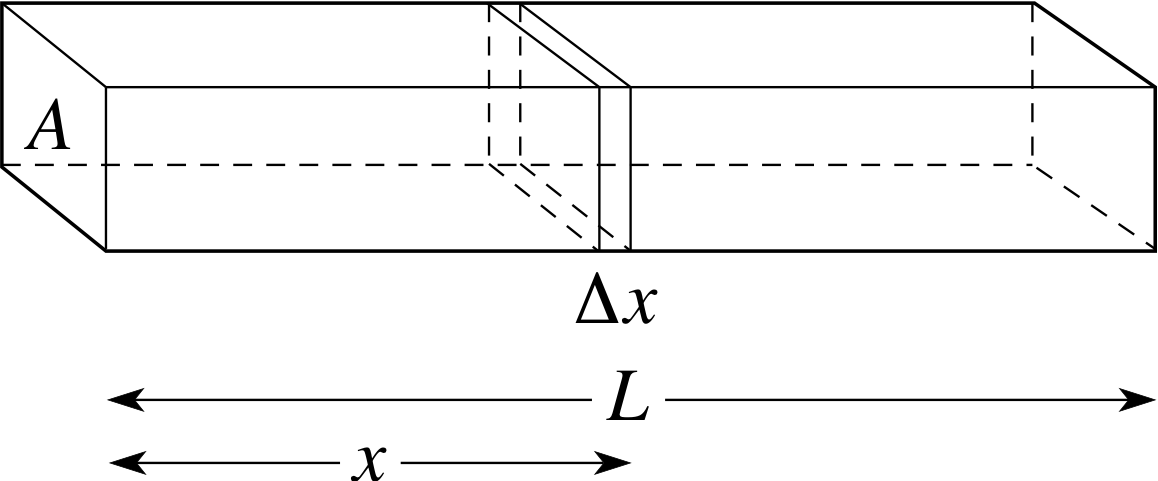
Figure 18 A rod of varying density.
Suppose that we want to find the mass of a rod of length L and uniform cross–sectional area A, whose density ρ (x) varies with distance x from one end of the rod (see Figure 18). We proceed by dividing the rod into thin slices of thickness ∆x. The volume of one of these slices is A ∆x, and since the density within this slice is approximately constant, and equal to ρ (x), the mass of the rod between x and x + ∆x is approximately ρ (x)A ∆x. The total mass M of the rod is approximately given by the sum of the masses of all the thin slices. In the limit as ∆x tends to zero, this sum becomes a definite integral, exactly equal to the mass of the rod:
$M = A\Int_0^L\rho(x)\,dx$(14)
✦ Find the mass M of a rod of length L and cross–sectional area A whose density is given by $\rho(x) = \dfrac{\rho_0}{L^2+x^2}$ where ρ0 is a constant.
✧ $\displaystyle M = A\int_0^L\dfrac{\rho_0}{L^2+x^2}\,dx = \dfrac{A\rho_0}{L}\left[\arctan(xL)\right]_0^L = \dfrac{A\pi\rho_0}{4L}$ from a table of standard integrals. i
(Alternatively the integral can be evaluated by the substitution x = L tan u.)
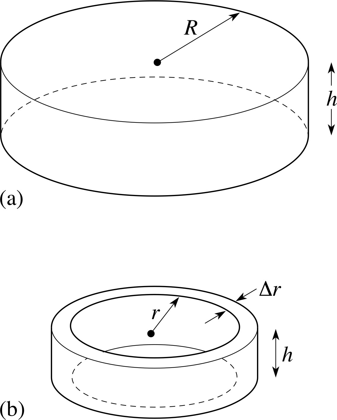
Figure 19 (a) A disc of varying density. (b) A thin ring–shaped portion of the disc.
The method used to derive Equation 14 can be generalized to find the mass of some solids which are not in the shape of rods. For example, suppose we want to find the total mass of a disc, of radius R and depth h whose density ρ (r) varies with the distance r from the axis of the disc (see Figure 19a). Since the density depends only on r, and on neither the angular displacement round the disc nor the depth, we can easily write down an approximate expression for the mass of a thin ring-shaped portion of the disc (shown in Figure 19b) if we know the volume of such a portion. We therefore divide the disc into thin concentric rings of radius r and thickness ∆r, calculate the mass of one such ring, and add up the masses of all the rings; then, as usual, as we let ∆r tend to zero, the resulting integral gives us the mass of the disc.
To find the mass of the ring, note that its volume is approximately equal to the product of its inner circumference 2πr, its thickness ∆r and its depth h. So that
mass of the ring = $\overbrace{\underbrace{2\pi r}_{\color{purple}{\large\substack{\text{circumference}\\[2pt]\text{of ring}}}} \underbrace{h}_{\color{purple}{\large\substack{\text{depth}\\[2pt]\text{of ring}}}}\underbrace{\Delta r}_{\color{purple}{\large\substack{\text{thickness}\\[2pt]\text{of ring}}}}}^{\color{purple}{\large\text{volume of ring}}}\underbrace{\rho(r)}_{\color{purple}{\large\substack{\text{density}\\[2pt]\text{of ring}}}}$
and the mass M of the whole disc is given by:
$M = 2\pi h\Int_0^Rr\rho(r)\,dr$(15)
Question T8
Use Equation 15 to find the mass of a disc of radius R = 4 cm and height h = 1 cm, whose density $\rho(r) = \rho_0\sqrt{1 + r^2/R^2}$ where ρ0 = 300 kg m−3.
Answer T8
Substituting $\rho(r) = \rho_0\sqrt{1 + r^2/R^2}$ in Equation 15,
$M = 2\pi h\Int_0^Rr\rho(r)\,dr$(Eqn 15)
we have $M = 2\pi h\rho_0\Int_0^Rr\sqrt{1 + r^2/R^2}\,dr$. The integral can be evaluated using the substitution u = 1 + r2/R2; then du = 2r dr, i.e. $r\,dr = \frac12R^2\,du$. When r = 0, u = 1 and when r = R, u = 2. So the integral becomes:
$M = 2\pi h\rho_0R^2\Int_1^2\sqrt{u\os}\,du = 2\pi h\rho_0R^2\left[\frac23u^{3/2}\right]_1^2 = \frac23\pi h\rho_0R^2\left(2^{3/2}-1\right)$
Putting in R = 4 cm, h = 1 cm and ρ0 = 300 kg m22 gives M = 1.84 × 10⁻² kg.
The same strategy can be used to find the mass of a sphere of radius R whose density ρ (r) depends only on the distance r from the centre of the sphere. Here, we divide the sphere into thin spherical shells of thickness ∆r, concentric with the sphere. The volume of such a shell is approximately equal to the surface area of its inner surface, 4πr2, multiplied by its thickness ∆r.
✦ Write down an approximate expression for the mass of this spherical shell.
✧ The shell has approximate volume 4πr2 ∆r and the density ρ (r) is approximately constant throughout the shell. So the mass is approximately 4πr2ρ (r) ∆r.
As ∆r tends to zero, we obtain an integral giving the mass M of the sphere:
$M = 4\pi{\large\int}_0^Rr^2\rho(r)\,dr$(16) i
Question T9
Due to the effects of gravity, the density ρ (r) of a star varies with distance r from the centre of the star. Assuming that the density of a spherical star of radius R is given by ρ (r) = ρ0(1 − r3/2R3) where ρ0 is a constant, use Equation 16,
$M = 4\pi\Int_0^Rr^2\rho(r)\,dr$(Eqn 16)
to calculate the mass of the star.
Answer T9
Substituting ρ (r) = ρ0(1 − r3/2R3) in Equation 16,
$M = 4\pi\Int_0^Rr^2\rho(r)\,dr$(Eqn 16)
we find that the mass M of the star is
$M = 4\pi\rho_0\Int_0^Rr^2\left(1-\dfrac{r^3}{2R^3}\right)\,dr = 4\pi\rho_0\left[\dfrac{r^3}{3}-\dfrac{r^6}{12R^3}\right]_0^R = \pi\rho_0R^3$
4.2 Centre of mass
If we have a set of particles of masses m i distributed at positions x0i along the x–axis, the position xc of the centre of mass of this set of particles is given by
$x_{\rm c} = \dfrac{{\large\sum}_im_ix_i}{{\large\sum}_im_i}$(17)
Suppose for example that we have three small spheres of lead of mass 0.1 kg, 0.15 kg and 0.2 kg, attached to a thin rod, made of aluminium, at distances 5 cm, 10 cm and 75 cm, respectively, from one end of the rod. The centre of mass is the point about which the rod will balance, i) and according to Equation 17 this point will be approximately
$\dfrac{5 \times 0.1 + 10 \times 0.15 + 75 \times 0.2}{0.1 + 0.15 + 0.2}\,{\rm cm} \approx 37.78\,{\rm cm}$
from one end. We are ignoring the mass of the aluminium rod in this calculation since it is presumed to be small in comparison to the other masses. i
If we remove the lead weights then we can no longer ignore the mass of the rod, in which case we are dealing with a mass distributed uniformly instead of a number of discrete masses. In the case of a uniform rod i, made of aluminium say, it is clear that it will balance about its centre point, but generally we may need to use integration to find the position of a centre of mass.
Figure 18 A rod of varying density.
Suppose, for example, that we want to find the centre of mass of the non–uniform rod shown in Figure 18, of length L, cross–sectional area A and density ρ (x) (which varies along the length of the rod). We divide the rod into slices of thickness ∆x, and now we may treat it as a number of discrete masses and apply Equation 17 to obtain an approximate expression for xc.
The mass of the slice between x and x + ∆x is approximately ρ (x)A ∆x; and now we multiply the mass of this slice by its x–coordinate, sum over all slices, and divide this sum by the sum of the masses of the slices:
$x_{\rm c} = \dfrac{{\large\sum}_ix\rho(x)A\,\Delta x}{{\large\sum}_i\rho(x)A\,\Delta x}$
As ∆x tends to zero, this ratio of sums becomes a ratio of integrals, and we obtain an exact value:
$x_{\rm c} = \dfrac{A\Int_0^Lx\rho(x)\,dx}{A\Int_0^L\rho(x)\,dx}$(18a)
The integral in the denominator here is (from Equation 14) equal to the mass M of the rod; so an alternative way to write Equation 18a is
$x_{\rm c} = \dfrac AM\Int_0^Lx\rho(x)\,dx$(18b)
✦ Use Equation 18a to find the position of the centre of mass of a rod with uniform cross section and of length L, whose density ρ (x) at a point a distance x from one end is given by ρ (x) = C (x2 + L2), where C is a constant.
✧ The factor A cancels out of Equation 18a.
$x_c = \dfrac{A{\large\int}_0^Lx\rho(x)\,dx}{A{\large\int}_0^L\rho(x)\,dx}$(Eqn 18a)
The integral
${\large\int}_0^Lx\rho(x)\,dx = C{\large\int}x(x^2+L^2)\,dx = C\left[\frac14x^4+\frac12x^2L^2\right]_0^L = \frac34CL^4$
and the integral
${\large\int}_0^L\rho(x)\,dx = C{\large\int}(x^2+L^2)\,dx =C\left[\frac13x^3+x^2L\right]_0^L = \frac43CL^3$
So$x_c = \dfrac{\frac34CL^4}{\frac43CL^3} = \dfrac{9}{16}L$,
i.e. the centre of mass is at a distance $\frac{9}{16}L$ from the less dense end of the rod (x = 0). i
4.3 Moment of inertia
When you try to push a heavy object, the difficulty increases with the object’s mass. On the other hand, if you try to rotate an object about an axis, i the difficulty increases with a quantity known as its moment of inertia about that axis. You may have seen pictures of someone having difficulty opening the massive doors of a bank vault; this is not usually because there is resistance in the hinges, but because the doors have a large moment of inertia about the axis of the hinges (and once you get the door started it is just as difficult to stop it). The mass of an object is simply one of its intrinsic properties; but while the moment of inertia is related to an object’s mass, it also depends crucially on the choice of axis. The moment of inertia of a telegraph pole about the axis of circular symmetry of the pole is relatively small, but its moment of inertia about an axis through one end of the pole, and perpendicular to the pole, is quite considerable.
The moment of inertia I of a set of point masses mi about a given axis is defined as N
$\displaystyle I = \sum_{i=1}^Nm_ir_i^2$(19)
where ri is the perpendicular distance of mass mi from the axis and N is the total number of masses.
Some objects are designed so as to have very large moments of inertia. For example a flywheel is constructed to be as massive and with as large a diameter as is convenient, with most of its mass as far from the axis as possible. We will see why such a design is sensible shortly.
✦ Two equal point masses of magnitude 5 kg are fastened to the ends of a ‘light’ metre rule. What is the approximate moment of inertia about an axis perpendicular to the rule (a) through its centre (b) through one end?
✧ If we ignore the mass of the rule, then using Equation 19,
$\displaystyle I = \sum_{i=1}^Nm_ir_i^2$(Eqn 19)
we have:
(a) the moment of inertia about an axis through its centre is
5 kg × (0.5 m)2 + 5 kg × (0.5 m)2 = 2.5 kg m2
whereas:
(b) the moment of inertia about an axis through one end is
5 kg × (0 m)2 + 5 kg × (1.0 m)2 = 5 kg m2
Finding the moment of inertia of a number of point masses is relatively easy. When the mass is distributed throughout an object we generally need to employ integration, but not in the following case.
✦ A flywheel is designed so that most of its mass M is distributed around the rim of the wheel, of radius R say. If you are designing a flywheel to have the greatest possible moment of inertia, i is it better to double the mass and keep the radius fixed or to double the radius and keep the mass fixed?
✧ The rim of the wheel consists of a large number of small sections, each of mass mi say, at the same distance R from the axis of the wheel, so the moment of inertia is $\sum m_iR^2 = MR^2$. If we double the mass of the wheel this becomes 2MR2. On the other hand, if we double the radius it becomes 4MR2, so the second option is better.
The following example is based on a similar idea.
Example 6
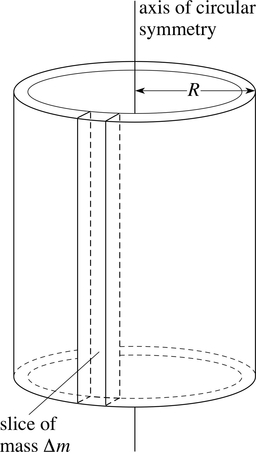
Figure 20 See Example 6.
Find the moment of inertia of a thin–walled hollow cylinder of radius R and mass M about its axis of circular symmetry (see Figure 20).
Solution
We divide the cylinder up into thin vertical slices each of mass ∆m. All points on such a slice have perpendicular distance r from the axis so, from Equation 19,
$\displaystyle I = \sum_{i=1}^Nm_ir_i^2$(Eqn 19)
the moment of inertia $I = \sum(\Delta m)R^2$. Since R2 is a constant, it can be taken
outside the summation sign, so that $I = R^2\sum\Delta m$. But $\sum\Delta m$ is simply equal to the total mass M of the cylinder, so
The moment of inertia of a thin hollow cylinder about the axis of the cylinder
I = MR2(20)
Note that this result does not depend on the height of the cylinder.
The previous cases were easy because the object could be divided into a number of small masses which were (approximately) the same distance from the axis; when the distance from the axis varies we will need to employ a more sophisticated summation process, which will lead to a definite integral. Here are some examples:
Thin rods
Example 7
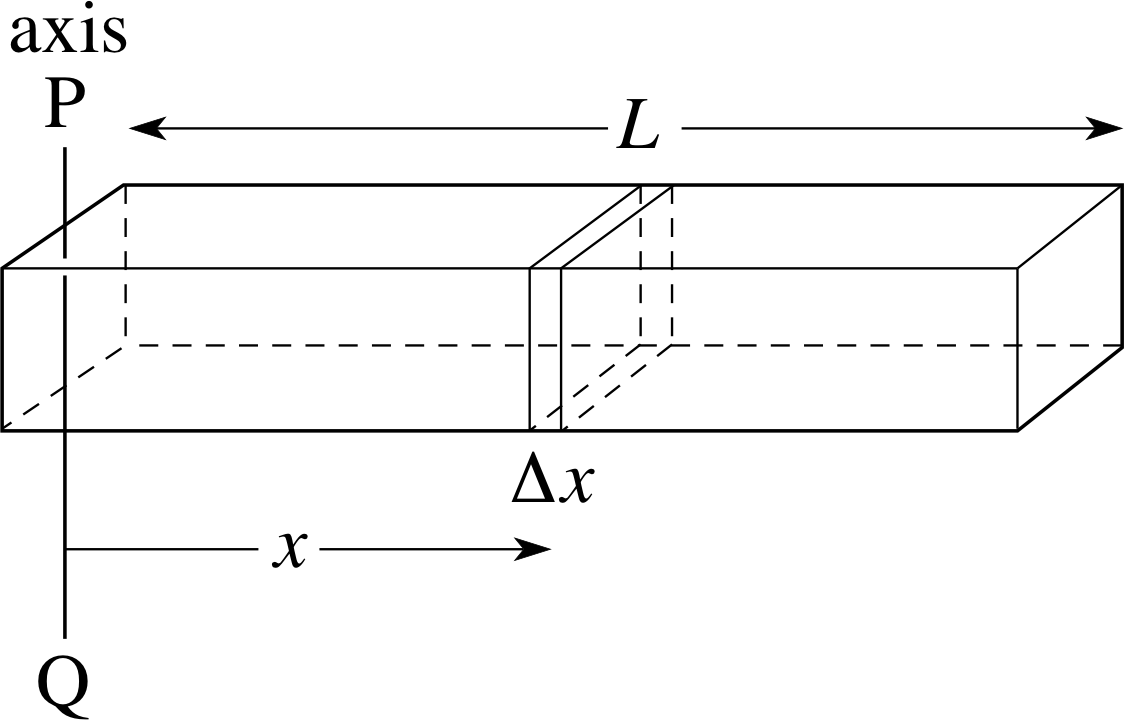
Figure 21 See Example 7.
Find the moment of inertia of a thin uniform rod (i.e. of constant cross–sectional area and uniform density), about an axis PQ perpendicular to the rod and passing through one end, in terms of its mass M and its length L (see Figure 21).
Solution
We divide the rod up into small slices of length ∆x. (Note that we have chosen the axis to be situated at the end x = 0 of the rod, which will make it easy to write down the distance of each slice from the axis.) As the rod is of uniform density and cross section, we can say that the mass per unit length of the rod is M/L, so that each thin slice has a mass
$\Delta M = \dfrac ML\Delta x$
Since the slice is presumed to be very thin, the perpendicular distance of all points within the slice from the axis is approximately x. i
We can now set up the integral we want to evaluate. The moment of inertia of each slice is approximately
$\underbrace{\dfrac ML\Delta x}_{\color{purple}{\large\substack{\text{mass of}\\[2pt] \text{slice}}}}~\underbrace{~~~x^2~~~}_{\color{purple}{\large\substack{\text{distance from}\\[2pt]\text{axis squared}}}}$
so the total moment of inertia of the rod is approximately ${\large\sum}\dfrac MLx^2\,\Delta x$. As ∆x tends to zero, this sum becomes an integral giving the moment of inertia I of the rod about the axis PQ:
$I = \dfrac ML{\Large\int}_0^Lx^2\,dx$
Evaluating this integral, we find
Moment of inertia of a rod about an axis through one end
$I = \dfrac ML\left[\dfrac13x^3\right]_0^L = \dfrac13ML^2$ i
Question T10
Find the moment of inertia of a thin uniform rod, of mass M and length L, about an axis perpendicular to the rod and passing through the centre of the rod. [Hint: Take the origin of coordinates to be at the centre of the rod.]
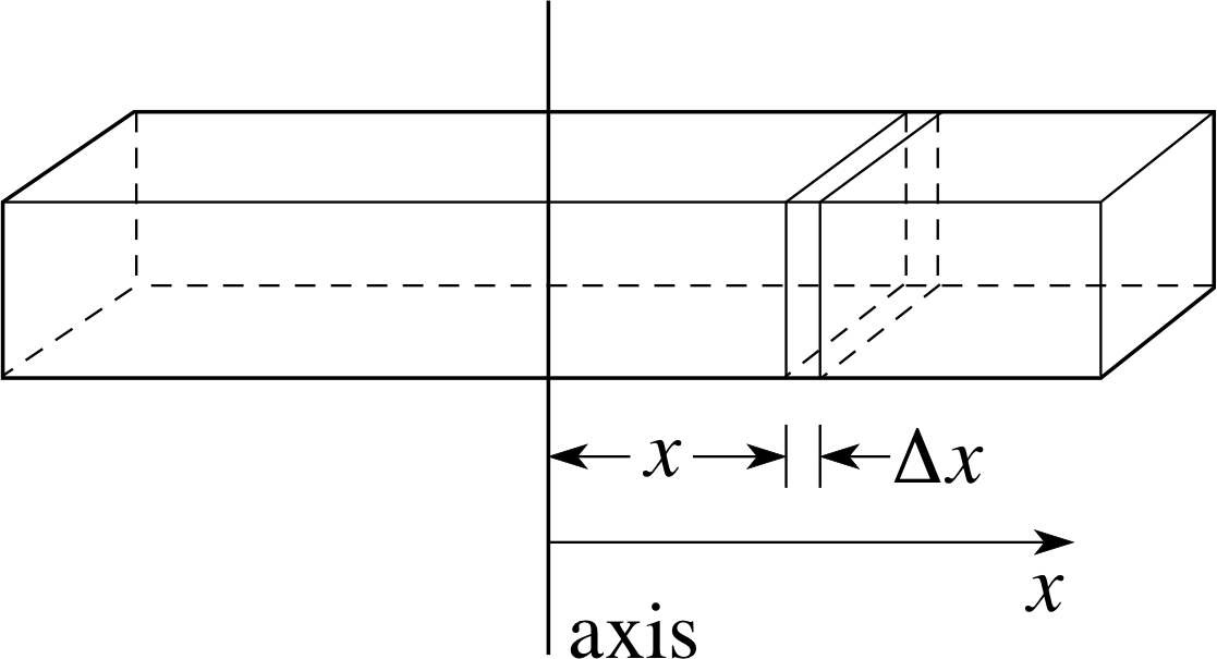
Figure 34 See Answer T10.
Answer T10
As in Example 7, the mass per unit length is M/L, so the mass of a slice of the rod of thickness ∆x is $\dfrac ML\Delta x$; the distance of such a slice from the axis
through the centre is x (see Figure 34) and so the integral to be evaluated is
$\dfrac ML\Int_{-L/2}^{L/2}x^2\,dx$
(the integrand is the same as in Example 7; only the limits are different). Evaluating the integral gives us
$I = \dfrac ML\left[\frac13x^3\right]{-L/2}^{L/2} = \frac{1}{12}ML^2$
Note that the moment of inertia about the axis through the centre is smaller than that about the axis through one end, as we would expect; in the first case, more of the rod is further from the axis.
This approach can easily be adapted to the case where the density of the thin rod is not constant, but varies along its length. Suppose that the rod in Example 7 has density ρ (x) at a distance x from one end, and constant cross–sectional area A.
Figure 21
✦ What is the moment of inertia of a thin slice of the rod of thickness ∆x about the axis PQ shown in Figure 21?
✧ The mass of this slice is ρ (x)A ∆x, and it is at a distance x from the axis. So its moment of inertia is
$\underbrace{\rho(x)\overbrace{A\,\Delta x}^{\color{purple}{\large\substack{\text{volume}\\\text{of slice}}}}}_{\color{purple}{\large\substack{\text{mass of}\\\text{slice}}}}\underbrace{x^2}_{\color{purple}{\large\substack{\text{distance from}\\\text{axis squared}}}}$
✦ Now write down an integral giving the total moment of inertia of the rod about the axis PQ.
✧ The required integral is
$A{\large\int}_0^L\rho(x)x^2\,dx$(21)
Question T11
A thin rod of length 10 cm and constant cross–sectional area 1.0 mm2 has density ρ (x) = B + Cx, where B = 250 kg m−3 and C = 330 kg m−4. Calculate its moment of inertia about an axis perpendicular to the rod, and passing through one end.
Answer T11
We use Equation 21,
$A{\large\int}_0^L\rho(x)x^2\,dx$(Eqn 21)
substituting ρ (x) = B + Cx. This gives us
$I = A\Int_0^L(B+Cx)x^2\,dx = A\left[\frac13Bx^3+\frac14Cx^4\right]_0^L = A(\frac13BL^3 +\frac14CL^4)$
With A = 1.0 mm2 = 10−6 m2, L = 10 cm = 0.1 m, B = 250 kg m−3, C = 330 kg m−4, we find
$I = 10^{-6}(\frac13\times 250\times(0.1)^3 + \frac14\times330\times(0.1)^4)\,{\rm kg\,m^2} = 9.16\times10^{-8}\,{\rm kg\,m^2}$
Solid cylinders and discs
Equation 20,
I = MR2(Eqn 20)
gives us the moment of inertia of a hollow cylinder about its axis of circular symmetry. We can use this result to calculate the moment of inertia of a solid cylinder of uniform density about its axis of circular symmetry (see Figure 22). We simply divide the cylinder into a large number of concentric thin–walled hollow cylinders, i use Equation 20 to write down the moment of inertia of a typical one of these, add up all such moments of inertia, and so arrive at an integral.
We first need to calculate the mass of a typical cylindrical shell of thickness ∆r, and, since we are assuming that the density of the cylinder is uniform, this just means finding the volume of the shell. Its volume is approximately equal to the product of its circumference (2πr), its thickness (∆r) and its height (h); so if the cylinder has density ρ,
∆M = the mass of a cylindrical shell = $\underbrace{~2\pi r~}_{\color{purple}{\large\text{circumference}}} \overbrace{~~h~~}^{\color{purple}{\large\text{height}}} \underbrace{~\Delta r~}_{\color{purple}{\large\text{thickness}}} \overbrace{~~\rho~~}^{\color{purple}{\large\substack{\text{constant}\\[2pt]\text{density}}}}$
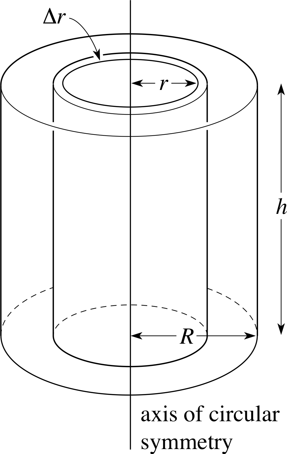
Figure 22 A solid cylinder of radius R and height h.
Its radius is r; so (replacing M by ∆M and R by r in Equation 20) we find that the moment of inertia of this hollow cylinder is
2πrhρ ∆r × r2 = 2πr3ρh ∆r
The total moment of inertia of the cylinder is therefore approximately given by:
$\sum 2\pi r^3\rho h\Delta r$.
As ∆r tends to zero, the sum becomes an integral, giving the moment of inertia I exactly:
$I = 2\pi \rho h\Int_0^Rr^3\,dr$
We evaluate the integral, to find
$I = 2\pi \rho h\left[\frac14r^4\right]_0^R = \frac12\pi\rho hR^4$(22)
It is usually more convenient to have an expression for I in terms of the mass M of the cylinder, rather than the density ρ. We know that the volume of the cylinder is πR2h so ρ = M/πR2h. Substituting for ρ in Equation 22 gives
$I = \frac12\pi hR^4 \times \underbrace{\left(\dfrac{M}{\pi R^2h}\right)}_{\color{purple}{\large{\text{density} \rho}}} = \frac12MR^2$
The moment of inertia of a uniform solid cylinder about its axis
$I = \frac12MR^2$(23)
Again, this result does not depend on the height of the cylinder (as in Equation 20),
I = MR2(Eqn 20)
and because of this, Equation 23 applies equally well to a thin disc as to a long cylinder.
If the density ρ (r) of the cylinder varies with distance r from its axis, the moment of inertia about the axis can also easily be written down as a definite integral. It is:
$I = 2\pi h\Int_0^Rr^3\rho(r)\,dr$(24)
where R and h are the radius and height of the cylinder.
Question T12
Derive Equation 24.
Answer T12
If the density of the cylinder varies with r, then the mass of the hollow cylinder shown in Figure 22 is approximately 2πrhρ (r) ∆r, so that its moment of inertia is approximately 2πr2hρ (r) ∆r. Adding these moments of inertia to obtain the total moment of inertia of the solid cylinder, and letting ∆r tend to zero gives the integral in Equation 24.
$I = 2\pi h\Int_0^Rr^3\rho(r)\,dr$(Eqn 24)
Solids of revolution
Since the height of the cylinder does not appear in Equation 23,
$I = \frac12MR^2$(Eqn 23)
that formula applies equally well to a thin disc as to a long cylinder. This means that we may use it to find the moment of inertia, about the x–axis, of any solid of revolution. We simply approximate the solid of revolution by a set of thin discs (as we did to find its volume), calculate the moment of inertia of one such disc using Equation 23, and, in the usual way, arrive at an integral.
Figure 12 Solid of revolution obtained by rotating the area under the graph of f (x) about the x–axis.
✦ Figure 12 shows an arbitrary solid of revolution, produced by rotating the area under the graph y = f (x) over the interval a ≤ x ≤ b about the x–axis. If the solid has uniform density ρ, find an expression for the moment of inertia of the disc D about the x–axis.
✧ The volume of the disc D is πy2∆x, so its mass is πy2ρ∆x. Its radius is equal to y, so from Equation 23,
$I = \frac12MR^2$(Eqn 23)
its moment of inertia about the x–axis is:
$\frac12\underbrace{\rho\pi y^2 \Delta x}_{\color{purple}{\large\text{mass of disc}}} \times \underbrace{y^2}_{\color{purple}{\large\substack{\text{radius of}\\\text{disc squared}}}} = \frac12\pi[f(x)]^4\rho\Delta x$
✦ Write down an integral giving the moment of inertia I about the x–axis of the solid of revolution in Figure 12.
✧
$I = \frac12\pi\rho{\large\int}_a^b[f(x)]^4\,dx$(25)
Example 8
Find the moment of inertia of a uniform sphere of radius R, density ρ and mass M about a diameter. (Give the answer in terms of M and R.)
Solution
Figure 13 See Example 8.
We recall first that a sphere of radius R is the solid of revolution obtained by rotating the semicircle $y = \sqrt{R^2 - x^2}$ about the x–axis (compare Example 4, and Figure 13).
Then the x–axis is a diameter of the sphere; so we may use Equation 25,
$I = \frac12\pi\rho\Int_a^b\left[\,f(x)\right]^4\,dx$(Eqn 25)
with $f(x) = \sqrt{R^2 - x^2}$, and limits of integration −R and R. This gives
$I = \frac12\pi\rho\Int_{-R}^R\underbrace{\left(R^2-x^2\right)^2}_{\color{purple}{\large{\left[\,f(x)\right]^4}}}\,dx = \frac12\pi\rho\Int_{-R}^R\left(R^4-2R^2x^2+x^4\right)\,dx$
$\phantom{I }= \frac12\pi\rho \left[R^4x-\frac23R^2x^3+\frac15\right]_{-R}^R = \frac{8}{15}\pi\rho R^5$
To express the answer in terms of R and M, we write $\rho = \dfrac{\rm{mass}}{\rm {volume}} = \dfrac{M}{\frac43\pi R^3}$, so that:
$I = \underbrace{\left(\dfrac{M}{\frac43\pi R^3}\right)}_{\color{purple}{\large{\text{density} \rho}}}$ $ \times \frac{8}{15}\pi R^5 = \frac25MR^2$.
Question T13
Find the moment of inertia about the axis of symmetry of a cone of radius r, uniform density ρ, height h and mass M. Give the answer in terms of M. [Hint: You may like to refer back to the calculation of the volume of a cone in Subsection 3.1.]
Figure 10 A cone of height h and base radius r.
Answer T13
We draw the cone as in Figure 10, and recall that the equation of the line OP is y = rx h. Substituting f (x) = rx/h in Equation 25,
$I = \frac12\pi\rho\Int_a^b\left[\,f(x)\right]^4\,dx$(Eqn 25)
and taking the limits of integration to be 0 and h, we find
$I = \frac12\pi\rho{\displaystyle \int}_0^h\dfrac{r^4}{h^4}x^4\,dx = \frac12\pi\rho\left[\dfrac{r^4}{5h^4}x^5\right]_0^h = \frac{1}{10}\pi\rho r^4h$
As the volume of this cone is $\frac13\pi r^2h$, $\rho = \dfrac{M}{\frac13\pi r^2h}$ and so we finally have
$I = \dfrac{M}{\frac13\pi r^2h} \times \frac{1}{10}\pi\rho r^4h = \frac{3}{10}Mr^2$
4.4 Function averages
In everyday language the word ‘average’ is a much abused term. Of course, we know roughly what we mean by saying ‘an average man’ or ‘an average day for the time of year’. We mean that the ‘man’ or ‘day’ is in some way a good representative of all men or days. In this subsection and the next we will discuss two forms of ‘average’ that are quite distinct, the point being that our choice of meaning for the word ‘average’ depends on the context. Our first illustration concerns average velocity.
You are probably familiar with the definition of average velocity between two times t1 and t2 as
$\dfrac{\text{total displacement between } t = t_1 \text{ and } t = t_2}{\text{total time } (t_2 - t_1)}$
In the case of an object travelling along the x–axis, we saw in Subsection 2.1 that if we know the velocity vx(t) as a function of time, we can find the total displacement between two times as an integral, $\Int_{t_1}^{t_2}v_x(t)\,dt$.
So, if we introduce the notation vav for average velocity, then
$v_{\rm {av}} = \dfrac{\Int_{t_1}^{t_2}v_x(t)\,dt}{t_2 - t_1}$ i
✦ The velocity vx(t) of an object at time t is given by vx(t) = at2. What is the average value of the velocity from t = 0 to t = T ?
✧
$v_{\rm av} = \dfrac{{\large\int}_0^Tat^2\,dt}{T-0} = \dfrac1T\left[\dfrac{at^3}{3}\right]_0^T = \dfrac13aT^2$
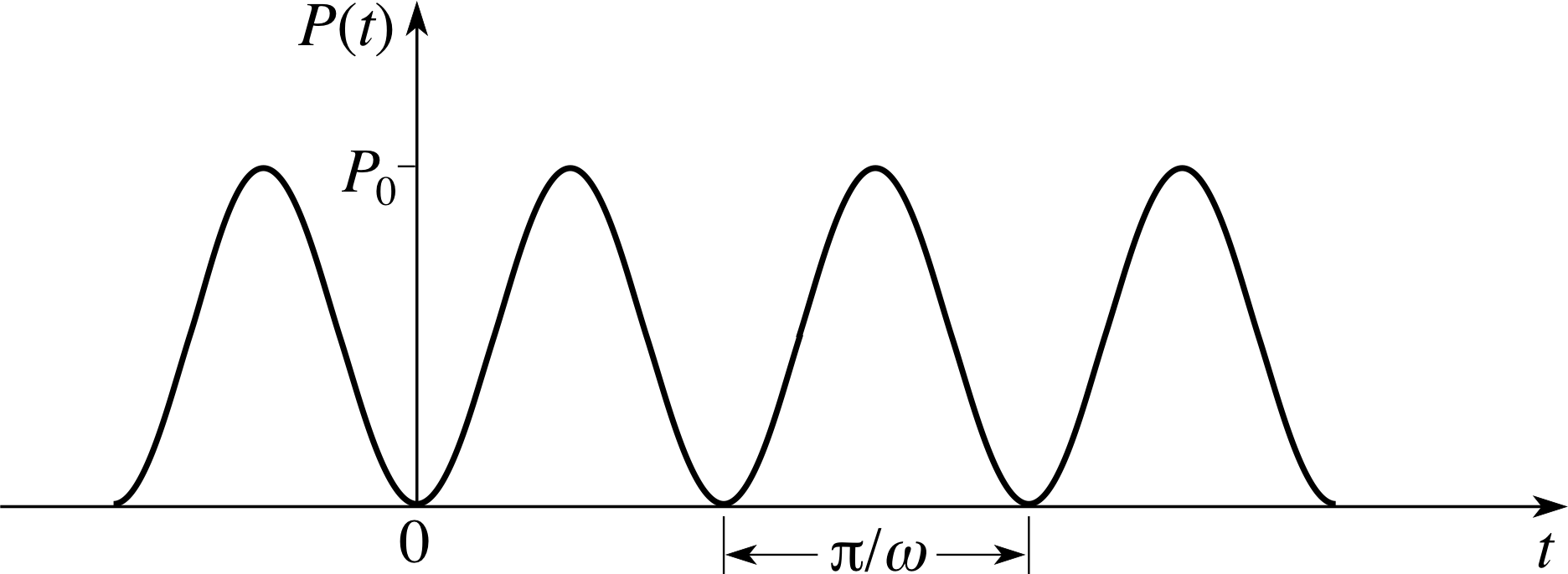
Figure 23 Sketch of P (t) = P0sin2 (ω0t).
We can use the same method to calculate average values of other functions. For example, consider the electrical power used by a domestic appliance. The power P supplied to a particular appliance by the mains in the United Kingdom is designed so that it varies with time according to the formula
P (t) = P0sin2 (ω0t)
where P0 is a constant depending on the power rating of the particular appliance.
A sketch of P against t is shown in Figure 23. The power rating quoted for any domestic appliance is actually defined to be the average power consumed. We can find an expression for this average power Pav in terms of P0 by calculating the average over just one cycle, since the symmetry of the graph means that the average over many cycles is the same as the average over one cycle.
So we will calculate the average power consumed between t = 0 and t = π/ω, which is given by the integral of P (t) between these times, divided by the time interval:
$P_{\rm av} = \dfrac{{\large\int_0^{\pi/\omega}}P(t)\,dt}{\pi/\omega - 0} = \dfrac{\omega}{\pi}{\large\int_0^{\pi/\omega}}P_0\sin^2(\omega t)\,dt$
To evaluate the integral, we use the trigonometric identity sin2(ωt) = ½ [1 − cos(2ωt)], so that
$P_{\rm av} = \dfrac{\omega P_0}{2\pi}{\large\int_0^{\pi/\omega}}\left[1-\cos(2\omega t)\right]\,dt = \dfrac{\omega P_0}{2\pi}\left[t-\dfrac{1}{2\omega}\sin(2\omega t)\right]_0^{\omega/\pi}$
and since sin 2π = sin 0 = 0, we finally find
$P_{\rm av} = \dfrac{\omega P_0}{2\pi} \times \dfrac{\pi}{\omega} = \dfrac{P_0}{2}$
So the average power is half the peak power P0.
So far in this subsection we have taken the integration variable to be time t, so that the averages in question were time averages. However, the notion of the average value of a function can be defined quite generally: for any function f (x), the average value fav over the interval a ≤ x ≤ b is defined as
$f_{\rm av} = \dfrac{\Int_a^bf(x)\,dx}{b-a}$(26)
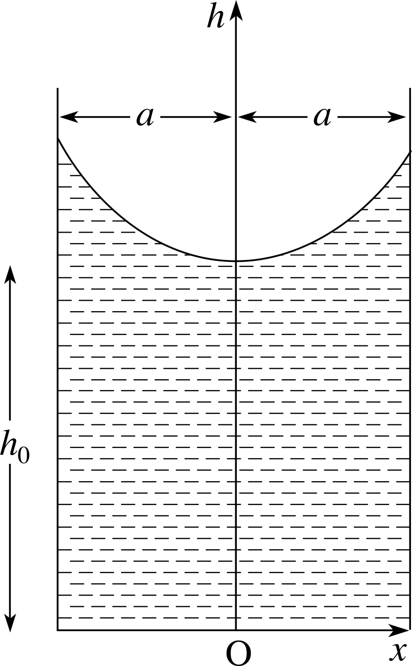
Figure 24 See Question T14.
Question T14
Figure 24 shows the cross section of a water surface between two glass plates. The height h of the water surface at position x is given by h (x) = h0 + bx2 for −a ≤ x ≤ a. Find the average height of the surface (i.e. the average value of h (x) over the interval −a ≤ x ≤ a).
Answer T14
From Equation 26, the average height of the surface is
$h_{\rm av} = \dfrac{\Int_a^b\left(h_0+bx^2\right)\,dx}{a-(-a)} = \dfrac{1}{2a}\left[h_0x+\dfrac b3x^3\right]_{-a}^a = \dfrac{1}{2a}\left(2h_0a+\dfrac{2b}{3}a^3\right) = h_0 + \dfrac{ba^2}{3}$
4.5 Mean value of a distribution
The word ‘average’ is often used in a completely different sense to the one introduced in Subsection 4.4. For example, if you sat three exams and scored 81% on the first, 52% on the second and 74% on the third, you might say that your ‘average score’ on all three was $\dfrac{\text{81% + 52% + 74%}}{3} = \text{69%}$. But it would be more correct to call this your mean score. Generally speaking, the mean of N numbers is defined as the sum of the numbers, divided by N. i
There are several different ways of writing an expression for a mean value. To illustrate the point, let us suppose that we have several, say N, particles moving with different constant speeds and we want to know the mean value $\langle v\rangle$ of their speeds. We measure the speed of each one, and find that N1 of them have speed v1, N2 have speed v2, and so on up to Nn having speed vn (so that N1 + N2 + ... + Nn = N, where n is the number of different speed groups). Instead of adding up the measured values one by one to obtain the mean value of all our measurements, we can multiply each of the n values obtained by the number of times it occurs, add the results, and divide by N. What we obtain is the mean_of_a_distributionmean value of the distribution:
$\displaystyle \langle v\rangle = \dfrac1N\sum_{i=1}^nN_iv_i$(27)
The fraction fi of times that the result vi occurs is simply Ni /N so we can rewrite Equation 27 in the form
$\displaystyle \langle v\rangle = \sum_{i=1}^n\,f_iv_i$(28)
(Notice that it follows that $\displaystyle \sum_{i=1}^n\,f_i = 1$ because N1 + N2 + ... + Nn = N.)
✦ Six particles have speeds 5 m s−1, 5 m s−1, 5 m s−1, 10 m s−1, 10 m s−1 and 20 m s−1. Use Equation 28 to calculate the value of $\langle v\rangle$.
✧ v1 = 5 m s−1 and f1 = 3/6 (this speed occurs 3 times in 6)
v2 = 10 m s−1 and f2 = 2/6
v3 = 20 m s−1 and f3 = 1/6
so that:
$\displaystyle \langle v\rangle = \sum_{i=1}^3 f_iv_i = (\frac36\times 5+\frac26\times10+\frac16\times20)\,{\rm m\,s^{-1}} \approx 9.17\,{\rm m\,s^{-1}}$
If we are interested, not in the mean speed, but in the mean value of some other physical quantity x, then this is given by an equation just like Equation 28:
$\displaystyle \langle x\rangle = \sum_{i=1}^n\,f_ix_i$(29)
where fi is the fraction of particles possessing the value xi of x, and i = 1, 2, 3, ... n.
✦ The speeds of a group of cars moving along a motorway are measured to the nearest 5 m s−1. 10% of the cars have speed 30 m s−1, 40% have speed 35 m s−1, 30% have speed 40 m s−1 and 20% have speed 45 m s−1. What is the mean speed of the cars?
✧ The mean speed is
(0.1 × 30 + 0.4 × 35 + 0.3 × 40 + 0.2 × 45) m s−1 = 38 m s−1.
Now suppose we are interested in finding the mean speed of molecules in a gas_phasegas. There are so many molecules that Equation 28, as it stands, is not going to be very useful to us; only a very small fraction of molecules will have any given speed, and we would have a very large number of speeds to sum over. Instead, what we do is divide up the range of all speeds available to the molecules into small intervals ∆v, and concentrate, not on the fraction fi of molecules with a particular speed vi but on the fraction of molecules with speeds lying within the small interval between v and v + ∆v. We expect this fraction to be proportional to the size ∆v of the interval, and we write it as f (v) ∆v. The function f (v) is known as a speed distributiondistribution function: it tells us what fraction of molecules have speed close to the value v.
We can then write Equation 28 as
$ \langle v\rangle = {\large\sum}v\underbrace{~\,f\,\Delta v~}_{\color{purple}{\large\substack{\text{fraction with}\\[2pt]\text{speed between }\\[1pt]v \text{ and } v+∆v}}}$
and, as we have done so often before in this module, we allow ∆v to tend to zero, so that the sum becomes an integral, and since there will be an upper bound, V say, to the speed of the molecules, we can write
$ \langle v\rangle = \Int_0^Vv\,f(v)\,dv$(30) i
An integral of this sort is far easier to perform than a sum over many different speeds, particularly when we know the specific form for the function f (v).
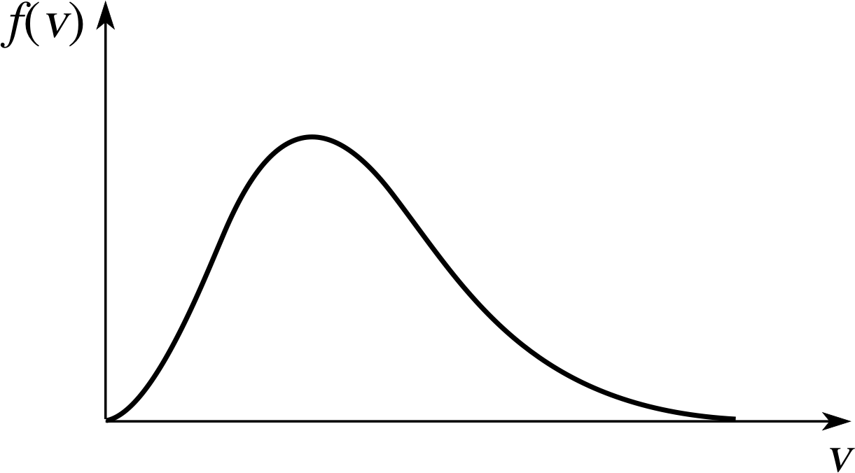
Figure 25 The Maxwell–Boltzmann speed distribution.
Remember that f (v) ∆v represents the fraction of molecules with speeds lying between v and v + ∆v, and all these fractions must sum to 1, in other words
$\Int_0^Vf(v)\,dv = 1$
The following function provides an appropriate mathematical model for f (v) molecules in a gas, and is known as the Maxwell–Boltzmann speed distribution:
$f(v) = 4\pi\left(\dfrac{m}{2\pi kT}\right)^{3/2}v^2\exp(-mv^2/2kT)$(31) i
where m is the mass of one of the molecules, T is the temperature of the gas, and k is Boltzmann’s constant. This speed distribution is sketched in Figure 25.
Question T15
Use the Maxwell–Boltzmann speed distribution in Equation 31 to calculate the mean speed v of molecules of mass m in a gas at temperature T. [Hint: You may find the substitution u = mv2/2kT helpful.]
Answer T15
From Equation 30,
$\langle v\rangle = \Int_0^Vv\,f(v)\,dv$(Eqn 30)
$\langle v\rangle$ is given by $4\pi\left(\dfrac{m}{2\pi kT}\right)^{3/2}\Int_0^\infty v^3\exp(-mv^2/2kT)\,dv$
With the substitution $u = \dfrac{mv^2}{2kT}$ we have du = kT dv, or v dv = m du; and $v^2\exp(-mv^2/2kT) = \dfrac{2kT}{m}u{\rm e}^{-u}$.
So$\langle v\rangle = 4\pi\left(\dfrac{m}{2\pi kT}\right)^{3/2}\Int_0^\infty \left(v^2\right)v\exp(-mv^2/2kT)\,dv$
So$\phantom{\langle v\rangle }= 4\pi\left(\dfrac{m}{2\pi kT}\right)^{3/2}{\displaystyle \int}_0^\infty\left(\dfrac{2kTu}{m}\right){\rm e}^{-u}\dfrac{kT}{m}\,du = 4\pi\left(\dfrac{m}{2\pi kT}\right)^{3/2}\times 2\left(\dfrac{kT}{m}\right)^2\Int_0^\infty u{\rm e}^{-u}\,du$
The value of this integral over u is given in the answer to Question R2, putting a = 1; it is equal to 1. Thus
$\langle v\rangle = 4\pi\left(\dfrac{m}{2\pi kT}\right)^{3/2}\times 2\left(\dfrac{kT}{m}\right)^2 \times 1 = \left(\dfrac{8kT}{\pi m}\right)^{1/2}$
In general, a distribution is a function which tells us what fraction of particles have values of a certain physical quantity lying in a particular small range: if we call the physical quantity X, then the distribution f (x) is defined so that
$f(x)\,∆x = \cases{\color{purple}{\text{fraction of particles with values of }X\\\text{in the interval between }x \text{ and }x + ∆x}\vphantom{p}}$(32)
The mean value x of X is then given by Equation 29,
$\displaystyle \langle x\rangle = \sum_{i=1}^n\,f_ix_i$(Eqn 29)
to be ${\large\sum}x\,f(x)\,\Delta x$, and, on allowing ∆x to tend to zero, the sum becomes an integral:
$x = \Int_a^bx\,f(x)\,dx$(33)
(where the limits of integration depend on the range of values that it is possible for x to take).
Example 9
The fraction of electrons in a metal near absolute zero with energies between E and E + ∆E is given by $\dfrac{3\sqrt{E\os}}{2E_{\rm F}^{3/2}}\,\Delta E$ for 0 ≤ E ≤ EF and is zero for E > EF, where EF is a constant known as the Fermi energy.
Verify that $\displaystyle \int_0^{E_{\rm F}}\dfrac{3\sqrt{E\os}}{2E_{\rm F}^{3/2}}\,dE = 1$ and find the mean energy of the electrons, in terms of EF.
Solution
The information given tells us about the energy distribution f (E) of the electrons; from Equation 32,
$f(x)\,∆x = \cases{\color{purple}{\text{fraction of particles with values of }X\\\text{in the interval between }x \text{ and }x + ∆x}\vphantom{p}}$(Eqn 32)
we see that
$f(E) = \dfrac{3\sqrt{E\os}}{2E_{\rm F}^{3/2}}$
for 0 ≤ E ≤ EF and f (E) = 0 for E > EF
First $\displaystyle \int_0^{E_{\rm F}}\dfrac{3\sqrt{E\os}}{2E_{\rm F}^{3/2}}\,dE =\dfrac{3}{2E_{\rm F}^{3/2}}\int_0^{E_{\rm E}}\sqrt{E\os}\,dE = \dfrac{3}{2E_{\rm F}^{3/2}}\left[\dfrac{2E^{3/2}}{3}\right] _0^{E_{\rm E}} = 1$
then substituting for f (E) into Equation 33 gives
$\displaystyle \int_0^{E_{\rm F}}\dfrac{3E^{3/2}}{2E_{\rm F}^{3/2}}\,dE = \dfrac{3}{2E_{\rm F}^{3/2}}\int_0^{E_{\rm E}}E^{3/2}\,dE = \dfrac{3}{2E_{\rm F}^{3/2}}\left[\dfrac{2E^{5/2}}{5}\right]_0^{E_{\rm F}} = \dfrac{3E_{\rm F}}{5}$
Question T16
The fraction of electrons in a metal near absolute zero with magnitude of momentum between p and p + ∆p is given by $\dfrac{3p^2}{p_{\rm F}^3}\,\Delta p$ for 0 ≤ p ≤ pF, and is zero for p > pF, where pF is a constant.Verify that $\displaystyle \int_0^{p_{\rm F}}\dfrac{3p^2}{p_{\rm F}^3}\,dp = 1$ and find the mean magnitude of momentum $\langle p\rangle$ of the electrons, in terms of pF.
Answer T16
The information given tells us about the momentum distribution f (p) of the electrons; from Equation 32,
$f(x)\,∆x = \cases{\color{purple}{\text{fraction of particles with values of }X\\\text{in the interval between }x \text{ and }x + ∆x}\vphantom{p}}$(Eqn 32)
we see that f (p) = 3 p2/pF3 for 0 ≤ p ≤ p2 and f (p) = 0 for p > p2.
First $\displaystyle \int_0^{p_{\rm F}}\dfrac{3p^2}{p_{\rm F}^3}\,dp = \dfrac{3}{p_{\rm F}}^3\left[\dfrac{p^3}{3}\right]_0^{p_{\rm F}} = 1$
then substituting for f (p) into Equation 30,
$ \langle v\rangle = \Int_0^Vv\,f(v)\,dv$(Eqn 30)
(with v replaced by p) gives:
$\langle p\rangle = \dfrac{3}{p_{\rm F}^3}{\displaystyle \int}_0^{p_{\rm F}}p^3\,dp = \dfrac{3}{p_{\rm F}}^3\left[\dfrac{p^4}{4}\right]_0^{p_{\rm F}} = \frac34p_{\rm F}$
Mean values also arise in quantum mechanics. Consider the case of a particle that can move along the x–axis. Unlike classical mechanics, quantum mechanics does not allow us to calculate the position x (t) of this particle as a function of time. Instead, all it can tell us is the probability P (x) ∆x of finding a particle on a small interval of the x–axis, between x and x + ∆x, at a given time. The function P (x) is known as a probability density.
Such functions must also have the property that $\Int_a^bP(x)\,dx =1$, since the probabilities must sum to 1.
If we know the probability density, we can use it to find the mean value which is defined as $\langle x\rangle$ of the position of the particle,
$\langle x\rangle = \Int_a^bxP(x)\,dx$(34)
where the limits of integration a and b depend on the region of the x–axis over which the particle is free to move.
Example 10
Consider a particle confined to move parallel to the x–axis between two ‘infinitely high walls’ at x = 0 and x = L. (Thus, however much kinetic energy the particle has, it can never escape from this region.) When the energy of this particle has the lowest value that is allowed by quantum mechanics, its probability density is $P(x) = \dfrac2L\sin^2\left(\dfrac{\pi x}{L}\right)$ for 0 ≤ x ≤ L and P (x) = 0 for | x | > L. First verify that this function is indeed suitable as a probability density, and then find the mean value of the particle’s position.
Solution
First we evaluate the integral $\displaystyle \int_0^LP(x)\,dx = \int_0^L\dfrac2L\sin^2\left(\dfrac{\pi x}{L}\right)\,dx$ note that, since the particle is confined to the region 0 ≤ x ≤ L the limits of integration are 0 and L. Using the trigonometric substitution sin2 y = ½ (1 − cos 2y) with y replaced by πx/L, we obtain
$\displaystyle \int_0^LP(x)\,dx = \dfrac1L\int_0^L\dfrac12\left[1 - \cos\left(\dfrac{2\pi x}{L}\right)\right]\,dx = \dfrac1L\left[x - \dfrac{L}{2\pi}\sin\left(\dfrac{2\pi x}{L}\right)\right]_0^L = 1$
which means that the function P (x) is suitable as a probability density. i
We now substitute the given probability density into Equation 34, to obtain $\displaystyle \langle x\rangle = \dfrac2L\int_a^bx\sin^2\left(\dfrac{\pi x}{L}\right)\,dx$. To evaluate the integral, we again use the trigonometric identity sin2 y = ½ (1 − cos 2y), which gives
$\displaystyle \langle x\rangle = \dfrac1L\int_0^Lx\left[1 - \cos\left(\dfrac{2\pi x}{L}\right)\right]\,dx = \dfrac1L\left[\dfrac12x^2\right]_0^L - \dfrac1L\int_0^Lx\cos\left(\dfrac{2\pi x}{L}\right)\,dx$(35)
We evaluate the remaining integral using integration by parts.
We find
$\displaystyle \int_0^Lx\cos\left(\dfrac{2\pi x}{L}\right)\,dx = \left[\dfrac{xL}{2\pi}\sin\left(\dfrac{2\pi x}{L}\right)\right]_0^L - \dfrac{L}{2\pi}\int_0^L\sin\left(\dfrac{2\pi x}{L}\right)\,dx$
$\displaystyle \phantom{\int_0^Lx\cos\left(\dfrac{2\pi x}{L}\right)\,dx }= \left[\dfrac{xL}{2\pi}\sin\left(\dfrac{2\pi x}{L}\right)\right]_0^L +\left(\dfrac{L}{2\pi}\right)^2\left[\cos\left(\dfrac{2\pi x}{L}\right)\right]_0^L$(36)
Since sin(2π) = sin 0 = 0 and cos(2π) = cos 0 = 1, the integral on the left–hand side of Equation 36 is in fact equal to zero. So, returning to Equation 35, we find
$\displaystyle \langle x\rangle = \dfrac1L\left[\dfrac12x^2\right]_0^L = \dfrac L2$
Question T17
When an electron in a hydrogen atom is in its state of lowest energy, the probability of finding it at a distance between r and r + ∆r from the nucleus is $(4/a_0^3)r^2\exp(-2r/a_0)\,\Delta r$, where a0 is a constant known as the Bohr radius; r may take any value between 0 and ∞. Verify that the function $P(r) = (4/a_0^3)r^2\exp(-2r/a_0)$ is suitable as a probability density, then use Equation 34,
$\langle x\rangle = \Int_a^bxP(x)\,dx$(34)
to find the mean value $\langle r\rangle$ of r.
Answer T17
The probability density $P(r) = \dfrac{4}{r^2}\exp(-2r/a_0)$ and, using integration by parts we find
$\Int_0^\infty P(r)\,dr = {\displaystyle \int}_0^\infty \dfrac{4}{r^2}{\rm e}^{-2r/a_0}\,dr = \dfrac{4}{a_0^3}\left\{\left[-\dfrac{a_0r^2}{2}{\rm e}^{-2r/a_0}\right]_0^\infty + \Int_0^\infty a_0{\rm e}^{-2r/a_0}\,dr\right\}$
The limits of integration are 0 and ∞ since r may lie anywhere between these values, and the first term on the
right-hand side above is zero, since r n exp(−2r/a0) tends to zero as r tends to infinity for any fixed value of n.
Therefore, from the answer to Question R2 with a = 2/a0, we have
$\Int_0^\infty P(r)\,dr = \dfrac{4}{a_0^3}\Int_0^\infty{\rm e}^{-2r/a_0}\,dr = 1$
Also, from Equation 34,
$\langle x\rangle = \Int_a^bxP(x)\,dx$(Eqn 34)
(with r replacing x), we have:
$\langle r\rangle = \Int_0^\infty rP(r)\,dr = \dfrac{4}{a_0^3}\Int_0^\infty r^3{\rm e}^{-2r/a_0}\,dr$
The integral over r can be evaluated by repeated application of integration by parts:
$\Int_0^\infty r^3{\rm e}^{-2r/a_0}\,dr = \left[-\dfrac{a_0}{2}r^3{\rm e}^{-2r/a_0}\right]_0^\infty + \dfrac{3a_0}{2}\Int_0^\infty r^2{\rm e}^{-2r/a_0}\,dr$
$\phantom{\Int_0^\infty r^3{\rm e}^{-2r/a_0}\,dr } = \underbrace{\left[-\dfrac{a_0}{2}r^3{\rm e}^{-2r/a_0}\right]_0^\infty}_{\color{purple}{\large\text{zero}}} + \underbrace{\dfrac{3a_0}{2}\left[-\dfrac{a_0}{2}r^2{\rm e}^{-2r/a_0}\right]_0^\infty}_{\color{purple}{\large\text{zero}}} + \dfrac{3a_0^2}{2}\Int_0^\infty r{\rm e}^{-2r/a_0}\,dr$
The remaining integral is given by the answer to Question R2, with a = 2/a0. So finally we find
$\Int_0^\infty r^3{\rm e}^{-2r/a_0}\,dr = \dfrac{3a_0^2}{2\os} \times \dfrac{1}{\left(2/a_0\right)^2} = \dfrac{3a_0^4}{8\os}$
and so
$\langle r\rangle = \dfrac{4}{a_0^3} \times \dfrac{1}{\left(2/a_0\right)^2} = \frac32a_0$
5 Closing items
5.1 Module summary
- 1
-
The Subsection 2.1area under the graph of f (x) between x = a and x = b is defined as being equal to the definite integral
$\Int_a^bf(x)\,dx$. This definition has the consequence that in any region where f (x) is always negative, so is the area under its graph. Sometimes we may be interested in the total size of the area enclosed by the graph of f (x) and the x–axis, between x = a and x = b (where a < b); this is given by the integral $\Int_a^b\lvert\,f(x)\rvert\,dx$
- 2
-
2 If the graphs of two functions f (x) and g (x) intersect at the points x = a and x = b (where a < b), then the Subsection 2.2area between the graphs is defined as
$\Int_a^b\lvert\,f(x) - g(x)\rvert\,dx$
This includes the case where other points of intersection lie between x = a and x = b.
- 3
-
A Section 3solid of revolution is a solid which can be obtained by rotating the area under a graph (or part of a graph) about some axis. If the solid is obtained by rotating the area under the graph of f (x) between x = a and x = b about the x–axis, then its volume (known as a volume of revolution) is given by the definite integral $\pi\Int_a^b\left[\,f(x)\right]^2\,dx$, and the area of its surface (known as a Subsection 3.2surface of revolution) is given by the definite integral
$S = 2\pi{\Large\int}_a^bf(x)\sqrt{1+\left[\,f'(x)\right]^2}\,dx$(13)
- 4
-
Integration may be used to find the mass M of a solid whose density ρ varies with position. In the case of a rod of constant cross–sectional area A and length L, lying along the x–axis between 0 and L, $M = A\Int_0^L\rho(x)\,dx$. For a disc of height h and radius R, whose density ρ (r) depends only on distance r from the axis, $M = 2\pi h\Int_0^Rr\rho(r)\,dr$. For a sphere of radius R, whose density ρ (r) depends only on distance r from the centre, $M = 4\pi\Int_0^Rr^2\rho(r)\,dr$.
- 5
-
The position of the Subsection 4.2centre of mass of a solid object may also be found by integration; for example, for a rod of constant cross–sectional area A and length L, lying along the x–axis between 0 and L, the x–coordinate of the Subsection 4.2centre of mass is $x_{\rm c} = M \Int_0^Lx\rho(x)\,dx$.
- 6
-
Subsection 4.3Moments of inertia of thin rods, solid cylinders, and solids of revolution can also be written as definite integrals.
The integral giving the Subsection 4.3moment of inertia I about the x–axis of the solid of revolution is
$I = \frac12\pi\rho\Int_a^b\left[\,f(x)\right]^4\,dx$(Eqn 25)
- 7
-
The Subsection 4.4average value of a function f (x) over the interval a ≤ x ≤ b is defined as
$f_{\rm av} = \dfrac{\Int_a^bf(x)\,dx}{b-a}$(Eqn 26)
- 8
-
A Subsection 4.5distribution is a function specifying the fraction of particles which have values of a certain physical quantity lying in a particular small range between x and x + ∆x; the distribution f (x) is defined so that this fraction is equal to f (x) ∆x where $\Int f(x)\,dx = 1$ and the mean of the distribution, $\langle x\rangle$, is given by a definite integral: $\langle x\rangle = \Int x\,f(x)\,dx$, where a and b are the largest and smallest allowed values of x, respectively.
5.2 Achievements
Having completed this module, you should be able to:
- A1
-
Define the terms that are emboldened and flagged in the margins of the module.
- A2
-
Interpret the definite integral of a given function between given limits in terms of the area under the graph of that function between those limits; and (paying due attention to signs) calculate the magnitude of the total area enclosed by the graph of the function and the horizontal axis.
- A3
-
Calculate the area enclosed between two intersecting graphs.
- A4
-
Write down definite integrals giving the volume and surface area of a solid of revolution.
- A5
-
Write down definite integrals giving the mass of a rod, disc or sphere whose density is not uniform.
- A6
-
Express the position of the centre of mass of a solid as a definite integral.
- A7
-
Find the moments of inertia of thin rods, cylinders, and solids of revolution as definite integrals.
- A8
-
Calculate the average value of a given function over a given interval.
- A9
-
Find the mean value of a distribution.
- A10
-
Use the idea of a definite integral as the limit of a sum in order to set up an integral that gives the value of some required physical quantity.
Study comment You may now wish to take the following Exit test for this module which tests these Achievements. If you prefer to study the module further before taking this test then return to the topModule contents to review some of the topics.
5.3 Exit test
Study comment Having completed this module, you should be able to answer the following questions, each of which tests one or more of the Achievements.
Question E1 (A2)
Calculate the area under the graph of f (x) = x2 − 8x + 12 between x = 0 and x = 6. Calculate also the sum of the magnitudes of the areas enclosed by the graph and the x–axis between x = 0 and x = 6. (You should start by sketching the graph.)
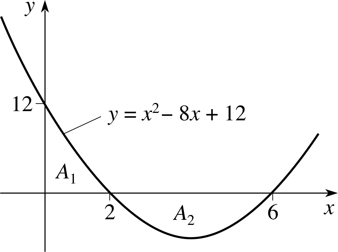
Figure 35 See Answer E1. (The horizontal and vertical scales are different in this figure.)
Answer E1
This quadratic function factorizes: f (x) = x2 − 8x + 12 = (x − 6)(x − 2). So the graph crosses the x–axis at x = 6 and x = 2, and we see that f (0) = 12.
The graph is sketched in Figure 35.
The area under the graph between x = 0 and x = 6 is
$\Int_0^6\left(x^2-8x+12\right)\,dx = \left[\frac13x^3-4x^2+12x\right]_0^6 = 0 - 0 = 0$
To find the magnitude of the area A1, we integrate between x = 0 and x = 2:
$A_1 = \Int_0^2\left(x^2-8x+12\right)\,dx = \left[\frac13x^3-4x^2+12x\right]_0^2 = \frac{32}{3} - 0 = 10.666$
Since we know that A1 + A2 = 0, it follows that A2 = −10.666; so the sum of the magnitudes of the areas enclosed by the graph and the x–axis is A1 + | A2 | = 10.666 + 10.666 = 21.333
(Reread Subsection 2.1 if you had difficulty with this question.)
Question E2 (A3)
Find the area between the graphs of f (x) = x2 − 2 and g (x) = 6 − x2.
Figure 36 See Answer E2.
Answer E2
The two graphs intersect where x2 − 2 = 6 − x2, i.e. x2 = 4. So the points of intersection are at x = −2 and x = 2.
The curves are sketched in Figure 36.
We see that g (x) is greater than f (x) within the range of integration; so the area between the graphs is given by
$\Int_{-2}^2\left[g(x)-f(x)\right]\,dx = \Int_{-2}^2\left(8-2x^2\right)\,dx = \left[8x-\frac23x^3\right]_{-2}^2 = 32-\frac{32}{2} = 21.33$
(Reread Subsection 2.2 if you had difficulty with this question.)
Question E3 (A4)
Find the volume and surface area of the solid of revolution obtained by rotating the area under the graph of f (x) = 2x between x = 2 and x = 4 about the x–axis.
Answer E3
The volume of revolution V is $\pi\Int\left[\,f(x)\right]^2\,dx$; with $f(x) = 2\sqrt{x\os}$ we have
$V = 4\pi\Int_2^4x\,dx = 4\pi\left[\frac12x^2\right]_2^4 = 4\pi(8-2) = 24\pi = 75.40$
The surface area S is $2\pi\Int_2^4f(x)\sqrt{1+\left[\,f'(x)\right]^2}\,dx$. With $f(x) = 2\sqrt{x\os}$ we have $f'(x) = 1/\sqrt{x\os}$. So the integrand is $2\sqrt{x\os} \times \sqrt{1 + 1/x\os} = 2\sqrt{x + 1\os}$, so
$S = 4\pi\Int_2^4\sqrt{x + 1\os}\,dx$.
We evaluate this integral by means of the substitution u = x + 1; then dx = du, the limits of integration become 3 and 5, and so
$S = 4\pi\Int_3^5u\,du = 4\pi\left[\frac23u^{3/2}\right]_3^5 = 4\pi(7.454-3.464) = 50.133$
(Reread Section 3 if you had difficulty with this question.)
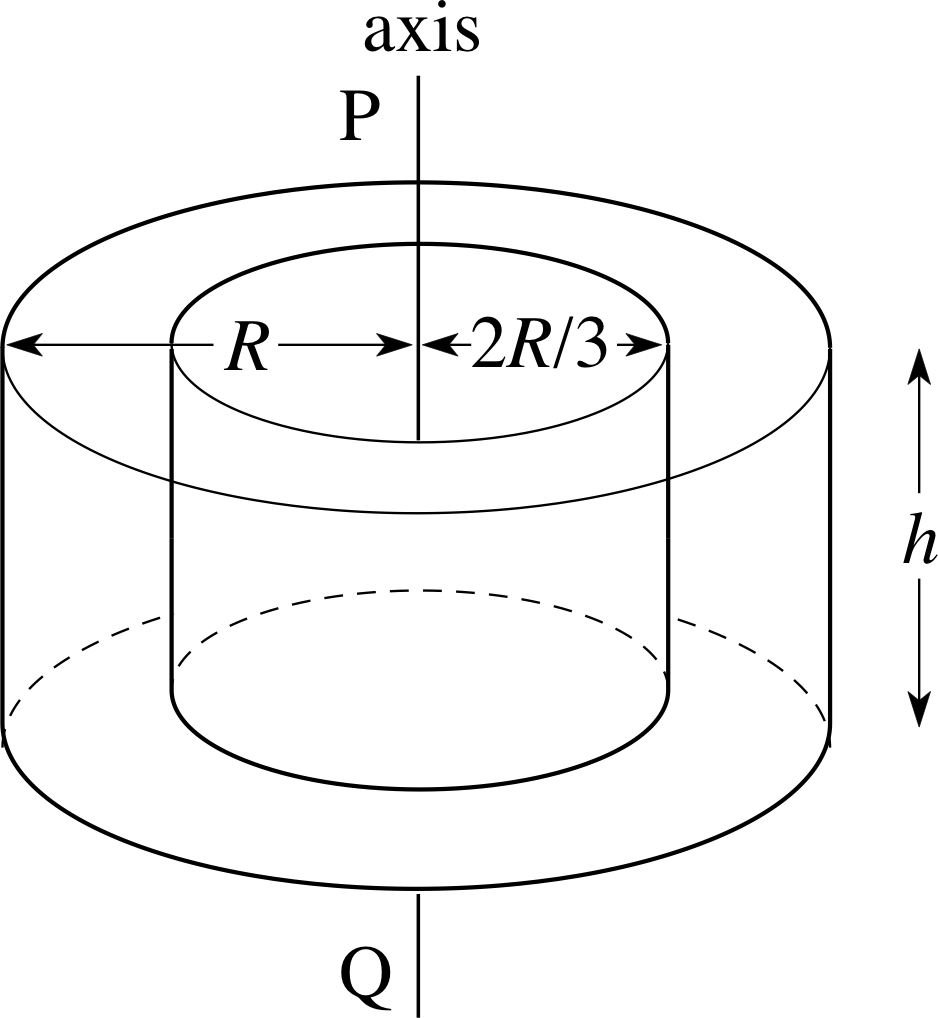
Figure 26 See Question E4.
Question E4 (A5 and A7)
The ring shown in Figure 26 has inner radius 2R/3, outer radius R and height h. Its density at any point at a perpendicular distance r from the axis PQ is $\rho(r) = \dfrac{\rho_0R^2}{r^2+R^2}$, where ρ0 is a constant. Find expressions for
(a) its mass M (in terms of ρ0, R and h), and
(b) its moment of inertia about the axis PQ (in terms of M and R).
Answer E4
We divide the ring up into narrow rings, of width ∆r. The mass of one such ring, with inner radius r, is approximately 2πrhρ (r) ∆r. Its moment of inertia about the axis PQ is approximately 2πr3hρ (r) ∆r.
(a) The mass M of the ring is
$\displaystyle 2\pi h\int_{2R/3}^Rr\rho(r)\,dr = 2\pi h\rho_0R^2\int_{2R/3}^R\dfrac{r}{r^2+R^2}\,dr$
The integral can be evaluated by means of the substitution u = r2 + R2; then du = 2r dr, or $r\,dr = \frac12du$. The limits of integration become $\frac{13}{9}R^2$ and 2R2, thus
$\displaystyle M = \pi h\rho_0 R^2\int_{13R^2/9}^{2R^2}\dfrac1u\,du = \pi h\rho_0 R^2\left[\loge u\right]_{13R^2/9}^{2R^2}\\ \phantom{M} = \pi h\rho_0 R^2\left[\loge(2R^2) - \loge(13R^2/9)\right] = \pi h\rho_0 R^2\loge \left(\dfrac{2}{13/9}\right) = \pi h\rho_0 R^2\loge \left(\dfrac{18}{13}\right) = 1.022h\rho_0 R^2$
(b) The moment of inertia I of the ring about the axis PQ is
$\displaystyle 2\pi h\int_{2R/3}^Rr^3\rho(r)\,dr = 2\pi h\rho_0R^2\int_{2R/3}^R\dfrac{r^3}{r^2+R^2}\,dr$
Again, the integral over r can be found with the substitution u = r2 + R2; the new limits of integration are as they were in part (a), and we have
$\displaystyle I = \pi h\rho_0 R^2\int_{13R^2/9}^{2R^2}\dfrac{u-R^2}{u}\,du = \pi h\rho_0 R^2\left[u - R^2\loge u\right]_{13R^2/9}^{2R^2}\\ \phantom{I} = \pi h\rho_0 R^2\left[2R^2 - \dfrac{13}{9}R^2 - R^2\loge \left(\dfrac{2}{13/9}\right) \right] = 0.723h\rho_0 R^4$
From the answer to part (a), we see that $h\rho_0 = \dfrac{M}{1.022R^2}$, so
$I = \dfrac{M}{1.022r^2} \times 0.723R^4 = 0.707MR^2$
(Reread Subsection 4.1Subsections 4.1 and Subsection 4.34.3 if you had difficulty with this question.)
Figure 16 Relation between slant height l, height h and radius r of a cone.
Question E5 (A6 and A10)
The cone shown in Figure 16 is the solid of revolution obtained by rotating the line y = rx/h about the x–axis between x = 0 and x = h. It is of uniform density. Find the position of its centre of mass.
Answer E5
By symmetry, the centre of mass must lie on the x–axis (the axis of the cone). To find its x–coordinate, we divide the cone into thin discs each of thickness ∆x, calculate the mass of a typical disc, and let ∆x tend to 0. As we allow ∆x to tend to zero, the sums in the numerator and denominator of our expression for xc will become definite integrals as in Equation 18,
$x_{\rm c} = \dfrac{A\Int_0^Lx\rho(x)\,dx}{A\Int_0^L\rho(x)\,dx}$(Eqn 18a)
The disc lying between x and x + ∆x has radius rx/h, so its volume is $\pi\left(\dfrac rh\right)^2x^2\,\Delta x$, and its mass is
$\rho\pi\left(\dfrac rh\right)^2x^2\,\Delta x$, where ρ is the density of the cone. Thus
$x_{\rm c} \approx \dfrac{\Sum\;\rho\pi\left(\dfrac rh\right)^2x^3\,\Delta x}{\Sum\;\rho\pi\left(\dfrac rh\right)^2x^2\,\Delta x} = \dfrac{\Sum\;x^3\,\Delta x}{\Sum\;x^2\,\Delta x}$
or, as ∆x tends to zero, $x_{\rm c} = \dfrac{\Int x^3\,\Delta x}{\Int x^2\,\Delta x}$
The integrals $\Int_0^hx^3\,dx = \left[\frac14x^4\right]_0^h = \frac14h^4\quad\text{and}\quad\Int_0^hx^2\,dx = \left[\frac13x^3\right]_0^h = \frac13h^3$, so
$x_{\rm c} = \dfrac{\frac14h^4}{\frac13h^3} = \frac34h$
(Reread Subsection 4.1Subsections 4.1 and Subsection 4.24.2 if you had difficulty with this question.)
Question E6 (A8)
The temperature T in a rod of length L is given by the equation $T(x) = \dfrac{T_0x}{L}\exp(-x^2/L^2)$, where x is the L distance from one end of the rod and T0 is a constant. What is the average temperature of the rod?
Answer E6
The average temperature Tav is given by
$T_{\rm av} = \dfrac{\Int_0^LT(x)\,dx}{L-0} = \dfrac{T_0}{L^2}{\displaystyle \int}_0^Lx\exp(-x^2/L^2)\,dx$
The integral can be evaluated by means of the substitution u = x2; then du = 2x dx, or $x\,dx = \frac12\,du$.
The new limits of integration are 0 and L2, so
$T_{\rm av} = \dfrac{T_0}{2L^2}{\displaystyle \int}_0^{L^2}\exp(-u/L^2)\,du = \dfrac{T_0}{2L^2}\left[-L^2\exp(-u/L^2)\right]_0^{L^2} = -\dfrac{T_0}{2}({\rm e}^{-1} - 1) = 0.316T_0$
(Reread Subsection 4.4 if you had difficulty with this question.)
Question E7 (A9)
The fraction of molecules in a gas with energies between E and E + ∆E is $\dfrac{2}{\sqrt{\pi\os}(kT)^{3/2}}\sqrt{E\os}{\rm e}^{-E/kT}\,\Delta E$, where T is the temperature of the gas, k is Boltzmann’s constant and E may take any positive value.
Given that $\displaystyle \dfrac{2}{\sqrt{\pi\os}(kT)^{3/2}}\int_0^\infty\sqrt{E\os}{\rm e}^{-E/kT}\,\Delta E = $, find the mean energy of a molecule. [Hint: Use integration by parts.]
Answer E7
The energy distribution of the molecules is
$f(E) = \dfrac{2}{\pi(kT)^{3/2}}\sqrt{E\os}{\rm e}^{-E/kT}$
and E may take any value between 0 and ∞. Since $\Int f(E)\,dE = 1$ the function is a suitable distribution function, so the mean energy is given by
$\langle E\rangle = \Int_0^\infty E\,f(E)\,dE = \dfrac{2}{\pi(kT)^{3/2}}\Int_0^\infty E^{3/2}{\rm e}^{-E/kT}\,dE$
Using integration by parts we have
$\Int_0^\infty E^{3/2}{\rm e}^{-E/kT}\,dE = \left[-kTE^{3/2}{\rm e}^{-E/kT}\right]_0^\infty + \dfrac{3kT}{2}{\displaystyle \int}_0^\infty\sqrt{E\os}{\rm e}^{-E/kT}\,dE = \dfrac{3kT}{2}\dfrac{\sqrt{\pi\os}(kT)^{3/2}}{2} = \dfrac{3\sqrt{\pi\os}(kT)^{5/2}}{4}$
So$\langle E\rangle =\dfrac{2}{\sqrt{\pi\os}(kT)^{3/2}} \times \dfrac{3\sqrt{\pi\os}(kT)^{5/2}}{4} = \frac32kT$
(Reread Subsection 4.5 if you had difficulty with this question.)
Study comment This is the final Exit test question. When you have completed the Exit test go back and try the Subsection 1.2Fast track questions if you have not already done so.
If you have completed both the Fast track questions and the Exit test, then you have finished the module and may leave it here.
Study comment Having seen the Fast track questions you may feel that it would be wiser to follow the normal route through the module and to proceed directly to the following Ready to study? Subsection.
Alternatively, you may still be sufficiently comfortable with the material covered by the module to proceed directly to the Section 5Closing items.