MATH 5.1: Introducing integration

3 The applications of integration

3.2 The stability of a satellite

5 Closing items

5.3 Exit test

Note that x, t and w are dimensionless variables in Questions F1 and F2. They have no physical significance in those questions.

In practice, derivatives are usually found by combining well–known ‘standard derivatives’ in a variety of ways, but both the standard derivatives and the rules for combining them are based on Equation 1.

Strictly speaking, position, velocity and acceleration are vector quantities in that each require three scalar_components_of_a_vectorscalar components for their complete specification in three dimensions. However, in the case of linear motion each of these quantities is effectively specified by a single scalar component. Thus, in the context of linear motion we will refer to x, v_x and a_x as position, velocity and acceleration, respectively, even though each is, in reality, only a single component of the corresponding vector.

Mention of newtons_laws_of_motionNewton’s laws, mass and force takes us beyond kinematics and into the realm of dynamics. These topics are fully discussed in the physics strand of FLAP, see the Glossary for details.

For reasons that will become clear later, inverse differentiation is usually referred to as indefinite integration.

Any other function of the form F(x) = x² + C, where C is any constant would be equally acceptable. C is then called an constant_of_integrationintegration constant or a constant of integration.

The constant K here represents the difference between the integration constants C₁ and C₂ associated with the inverse derivatives F₁(x) and F₂(x), i.e.K = C₁ −C₂.

Note that in this case we have used additional information about the problem, the condition v_x(0) = 0, to determine the relevant value of C. This is often necessary in physical problems.

In fact, g varies with distance from the centre of the Earth, and takes slightly different values at different places on the Earth’s surface. However, provided we consider a reasonably narrow range of vertical heights and restrict our attention to one locality it is reasonable to treat g as a constant.

Note the distinction between displacement and distance: in one dimension displacement may be positive or negative according to direction, but distance must always be positive.

If x is a positive quantity then |x| = x and |−x| = x.

The physical significance of simple harmonic motion is discussed in detail in the physics strand of FLAP.

ω is the Greek letter omega.

You can confirm that this is correct by showing that its derivative is −Aω²sin(ωt).

By combining Equations 10 and 12 it is possible to characterize simple harmonic motion by the requirement that a_x = −ω²x. This is the usual starting point for the analysis of simple harmonic motion and is considered elsewhere in FLAP. See the Glossary for details.

The shaded area in Figure 1b is a trapezium, the area of which is generally given by

$\frac12(\text{height}_1 + \text{height}_2) \times \text{base}$

Note that whichever inverse derivative of f(x) we choose to use when evaluating the area under the graph, the associated constant of integration C will play no part in the final answer since it will cancel when we calculate the difference F(b) − F(a).

The symbol ≈ means ‘approximately equal to’.

Here we are using the definition of the derivative to justify saying

$\displaystyle \begin{align}\lim_{\Delta x\rightarrow 0}{\left(\dfrac{\Delta A}{\Delta x}\right)} & = \lim_{\Delta x\rightarrow 0}{\left[\dfrac{A(x+\Delta x)-A(x)}{\Delta x}\right]}\\ & = \dfrac{dA}{dx}\end{align}$

Remember, the distance between two points is equal to the magnitude_of_a_vector_or_vector_quantitymagnitude of the displacement from one point to the other.

The symbol ≤ should be read as ‘is less than or equal to’.

Note that we have used the summation symbol (Σ) as a shorthand way of indicating the sum.

Notice that, while it is not essential that the points dividing the interval are equally spaced, it is very convenient if they are.

In this case a very crude approximation, since the actual value of the integral is 24.

The extension x increases from 0 to L, and we imagine this interval to be divided into a large number of subintervals by points x₁, x₂, ..., x_n + 1 where x₁ = 0 and x_n + 1 = L. The sum

$\displaystyle \sum_{i=1}^nF_x(x_i)\Delta x_i$

is thus a good approximation to the work done if the ∆x_i are small. With practice it is unnecessary to write down this intermediate step, and we go straight to the integral as in this example.

As you perform more and more integrals this result will become very familiar. Nonetheless it is worth pausing to note how remarkable it is that the limit of a sum represented by the symbol on the left can be evaluated with the aid of (inverse) differentiation as shown by the difference on the right. The link between summation and differentiation is far from obvious to most physicists.

Notice that $\displaystyle \int_1^3t^4\,dt$ is defined to be a limit of a sum – we can evaluate it using inverse differentiation.

You can confirm this by differentiating.

This notation arises from the fundamental theorem of calculus, from which it is evident that definite integrals are closely related to inverse derivatives.

The density is defined as the mass per unit volume.

This force acts perpendicular to the dam wall.

The angular brackets $\langle~\rangle$ mean ‘the average of’ the term enclosed.

If you imagine the arrow in Figure 10a rotating through 360° and carrying the satellite with it, then you can see that the satellite must also rotate through 360°.

You might have anticipated this result since in Figure 10b the section of the satellite to the left of centre is brought nearer to the Earth and so will be pulled further in this direction – not compensated sufficiently by the other half of the satellite, on which the force is weakened, as it is further from the Earth.

This statement is true for the functions treated in this module, but the definition of the definite integral as the limit of a sum allows it to be applied in cases where simple graphical interpretation is not possible.

exp(a) is an alternative way of writing e^a.

1 Opening items

1.1 Module introduction

The notion of a limit of a sum arises in many applications of mathematics to physics. For example, suppose we want to find the total mass of a cylindrical column of air, the density of which decreases with height in a known way. One approach is to divide the air column into a number of horizontal discs – like a stack of coins – each sufficiently thin that we may regard it as having constant density. We can then work out the mass of each disc by multiplying its volume by its (constant) density, and add all those disc masses together to find an approximate value for the mass of the entire column. Our final answer will only be an approximation to the correct value because our assumption that each disc has constant density is only approximately true. Nonetheless, we may obtain a good estimate in this way and we may improve its accuracy by increasing the number of discs in the sum. Indeed, if we consider what happens as the thickness of the discs approaches zero (and the number of discs approaches infinity) then we see that the limit of the sum of disc masses is the exact value of the air column’s total mass. This is typical of the way in which the limit of a sum may arise in a physical problem. Limits of sums of this kind are referred to by physicists and mathematicians as definite integrals. The formulation of physical problems in terms of definite integrals is a major theme of this module.

Another major theme is the evaluation of definite integrals. Sometimes the only way of evaluating the limit of a sum is to perform the sum for a very large number of terms and then try to work out what would happen ‘in the limit’ as the number of terms approached infinity. This ‘head-on’ approach called numerical integration can provide accurate answers, but it can also be time consuming and very hard work. Fortunately there are many situations in which the evaluation of definite integrals can be performed more easily thanks to an important mathematical result known as the fundamental theorem of calculus. According to the fundamental theorem there is a remarkable link between the evaluation of the limit of a sum and the process of differentiation. In fact, many definite integrals may be evaluated by a procedure in which the key step amounts to little more than the reversal of the usual process of differentiation. This process of inverse differentiation, or indefinite integration as it is more commonly called, is a vital part of the mathematical tool kit of every physicist and engineer.

In Section 2 of this module we introduce the basic concepts of definite and indefinite integration. We start by recalling the definition of a derivative and then go on to define the inverse derivative that emerges from the process of inverse differentiation. Using the physical concepts of position, velocity and acceleration we show how inverse derivatives may be used to evaluate quantities such as the distance travelled in a given time by an object moving with varying velocity. This discussion leads us to formulate the concept of a definite integral defined as the limit of a sum. We then state (and prove) the fundamental theorem of calculus which provides the formal link between the evaluation of limits of sums and inverse differentiation. Finally, we round off the section by explaining why it makes sense to refer to inverse derivatives as indefinite integrals.

Section 3 is concerned with the formulation of problems in terms of definite integrals and their evaluation using indefinite integrals. Section 4 attempts to put the topic into its scientific context and provides some exercises for you to do.

Study comment Having read the introduction you may find that you are already familiar with the material covered by this module and that you do not need to study it. If so, try the following Fast track questions. If not, proceed directly to the Subsection 1.3Ready to study? Subsection.

1.2 Fast track questions

Study comment Can you answer the following Fast track questions? If you answer the questions successfully you need only glance through the module before looking at the Subsection 5.1Module summary and the Subsection 5.2Achievements. If you are sure that you can meet each of these achievements, try the Subsection 5.3Exit test. If you have difficulty with only one or two of the questions you should follow the guidance given in the answers and read the relevant parts of the module. However, if you have difficulty with more than two of the Exit questions, you are strongly advised to study the whole module.

Question F1

Evaluate the following indefinite integrals: i

(a) ${\large \int}(1+2x+3x^2)\,dx$, (b) ${\Large \int}\left[\sin(2x) + \cos(3x)\right]\,dx$ (c) $\displaystyle \int\left({\rm e}^t + \dfrac{1}{t^2}\right)\,dt$, (d) ${\large \int}dw$

Answer F1

(a) ${\large \int}(1+2x+3x^2)\,dx = x+x^2+x^3+C$

where C is an arbitrary constant, since

$\dfrac{d}{dx}(x+x^2+x^3+C) = 1 + 2x + 3x^2$

(b) ${\large\int}\left[\sin(2x) + \cos(3x)\right]\,dx = -\frac12\cos(2x) +\frac13\sin(3x) + C$

where C is an arbitrary constant, since

$\dfrac{d}{dx}\left[-\frac12\cos(2x) +\frac13\sin(3x) + C\right] = \sin(2x) + \cos(3x)$

(c) ${\LARGE\int}\left({\rm e}^t + \dfrac{1}{t^2}\right)\,dt = {\large\int}({\rm e}^x + t^{-2})\,dt = {\rm e}^x - t^{-1} + C = {\rm e}^t + \dfrac1t + C$

where C is an arbitrary constant, since

$\dfrac{d}{dx}\left({\rm e}^t + \dfrac1t + C\right) = {\rm e}^t + \dfrac{1}{t^2}$

(d) ${\large\int}dw= {\large\int}1\,dw = w + C$

where C is an arbitrary constant, since

$\dfrac{d}{dx}(w + C) = 1$

Question F2

Evaluate the following definite integrals:

(a) ${\Large\int}_{-1/4}^{1/4}\cos(2\pi x)\,dx$, (b) ${\Large\int}_0^3(2t -1)^2\,dt$, (c) $\displaystyle \int_1^2\dfrac{\left(1+{\rm e}^t\right)^2}{{\rm e}^2}\,dt$, (d) $\displaystyle \int_4^9\sqrt{x\os}\left(x - \dfrac1x\right)\,dx$

Answer F2

(a) ${\Large\int}_{-1/4}^{1/4}\cos(2\pi x)\,dx = \left[\dfrac{\sin(2\pi x)}{2\pi}\right]_{-1/4}^{1/4} = \dfrac{1}{2\pi}\left[\sin\left(\dfrac{\pi}{2}\right) - \sin\left(\dfrac{-\pi}{2}\right)\right] = \dfrac{1}{2\pi}\left[1 - (-1)\right] = \dfrac{1}{\pi}$

(b) ${\Large\int}_0^3(2t -1)^2\,dt = {\Large\int}_0^3(4t^2 - 4t + 1)\,dt = \left[\dfrac43t^3 - 2t^2+t\right]_0^3 = \left(\frac43\times 27-18+3\right) - 0 = 36-18+3 = 21$

(c) $\displaystyle \int_1^2\dfrac{\left(1+{\rm e}^t\right)^2}{{\rm e}^t}\,dt = \int_1^2\dfrac{\left(1+2{\rm e}^t+{\rm e}^{2t}\right)^2}{{\rm e}^t}\,dt = \int_1^2({\rm e}^{-t}+2+{\rm e}^t)\,dt = \left[-{\rm e}^{-t}+2t+{\rm e}^t\right]_1^2~~~({\text{since}}~\dfrac{d}{dt}{\rm e}^{kt} = k{\rm e}^{kt})$

$ = (-{\rm e}^{-2} + 4 + {\rm e}^2) - (-{\rm e}^{-1} + 2 + {\rm e}) = {\rm e}^2 - {\rm e}^{-2} + {\rm e}^{-1} - {\rm e} + 2$

(d) $\displaystyle \int_4^9\sqrt{x\os}\left(x - \dfrac1x\right)\,dx = \int_4^9\left(x^{3/2} - x^{-1/2}\right)\,dx = \left[\dfrac25x^{5/2} - 2x^{1/2}\right]_4^9~~~({\text{since}}~\dfrac{d}{dx}\left(\dfrac{x^n}{n}\right) = x^{n-1}~if~n \ne 0)$

$ = \left(\dfrac25\times 3^5-6\right) - \left(\dfrac25\times 2^5-4\right) = \dfrac25(3^5-2^5) = \dfrac{412}{5} = 82.4$

Question F3

An object starts from rest at time t = 0, and moves along the x–axis with acceleration a_x(t) given, at time t, by

a_x(t) = a − bt where a = 5 m s⁻² and b = 3 m s⁻³

State whether each of the following statements is true or false and explain why.

(a) The object comes to rest when t = (5/3) s

(b) The displacement of the object from its initial position is zero when t = 5 s.

(c) The magnitude of the area bounded by the velocity–time graph and the t–axis, from t = 0 to t = 1 s, represents the distance the object travels in the first second.

(d) The magnitude of the area bounded by the graph of y = a_x(t) and the t–axis between t = 0 s and t = 5/3 s represents the maximum speed of the object in the first ten seconds.

Answer F3

Since a_x(t) = a − bt, where a = 5 m s⁻² and b = 3 m s⁻³, the velocity is

$v_x(t) = {\large\int}a_x(t)\,dt = {\large\int}(a-bt)\,dt = at - \dfrac{bt^2}{2} + C = \dfrac t2(2a-bt) + C$

for some particular constant C. But v_x = 0 when t = 0, so C = 0 and

$v_x(t) = \dfrac t2(2a - bt)$

Similarly, the position is given by

$x(t) ={\large\int}v_(t)\,dt = {\LARGE\int}\left(at-\dfrac{bt^2}{2}\right)\,dt = \dfrac{at^2}{2} - \dfrac{bt^3}{6}+D = \dfrac{t^2}{6}(3a-bt)+D$

where D is some particular constant.

(a) False. The velocity v_x is zero when t = 0 and again when t = 2a/b = (10/3) s.

(b) True. The position x is D when t = 0 and again when t = 3a/b = 5 s. It follows that the displacement (i.e. the difference in position) from the initial position is zero when t = 5 s.

(c) True. Generally the area under the velocity–time graph between two values of t represents the change in position (which may be positive or negative) over that time interval, rather than the distance moved (which must be positive). However in this case the velocity is positive in the time interval under consideration so the two are identical.

(d) False. Speed (a positive quantity) is the magnitude of velocity (which may be positive or negative). The area under the acceleration–time graph between two values of t represents the change in the velocity of the object over that time interval, so, since the velocity is zero when t = 0, the area from t = 0 to t = (5/3) s represents the velocity when t = (5/3) s. At this time the acceleration is zero, and the velocity attains a value of 4.167 m s⁻¹ (which happens to be its positive maximum). However, this does not represent the maximum speed. The velocity becomes negative when t exceeds (10/3) s, and subsequently stays negative becoming ever larger in magnitude. The velocity when t = 10 s is −100 m s⁻¹ so the speed at that time is 100 m s⁻¹, which clearly exceeds the speed at t = (5/3) s.

Study comment Having seen the Fast track questions you may feel that it would be wiser to follow the normal route through the module and to proceed directly to the following Ready to study? Subsection.

Alternatively, you may still be sufficiently comfortable with the material covered by the module to proceed directly to the Section 5Closing items.

1.3 Ready to study?

Study comment In order to study this module you will need to be familiar with the following terms: Cartesian coordinate system, derivative (or derived function), function, graph, limit, magnitude_of_a_vector_or_vector_quantitymagnitude (of a vector, as in magnitude_of_a_vector_or_vector_quantitymagnitude of a force), summation symbol (i.e. Σ). You should be able to differentiate a range of functions, and be able to expand, simplify and calculationevaluate expressions, including those that involve exponential_functionexponential and trigonometric functions. If you are uncertain of any of these terms, you can review them by referring to the Glossary which will indicate where in FLAP they are developed.

In particular you will need to know the following derivatives:

$\dfrac{d}{dt}(t^n) = nt^{n-1},~\dfrac{d}{dx}\left[\sin(at)\right] = a\cos(at),~\dfrac{d}{dt}\left[\cos(at)\right] = -a\sin(at),~\dfrac{d}{dt}({\rm e}^{at}) = a{\rm e}^{at}$

(where n and a are constants); and to remember that a function f(x) is often given by a formula such as y = f(x), and is a rule that assigns a unique value of y to each value of x (see the note below). The following questions will allow you to establish whether you need to review some of the topics before embarking on this module. Throughout this module $\sqrt{x\os}$ will represent the positive square root of x.

A special note on functions The function

f(x) = 1 + x + x²

is an example of a function that is defined for all values of x. One may think of the function as a sort of machine with x as the input and 1 + x + x² as the output. The input x is known as the independent variable and, if we write y = f(x), the output y is known as the dependent variable, since the function f(x) determines the way in which y depends on x.

The same function f could equally well be defined using some other symbol, such as t, to represent the independent variable:

f(t) = 1 + t + t²

This freedom to relabel the independent variable is often of great use, though it is vital that such changes are made consistently throughout an equation.

We may evaluate this function, whether we call it f(x) or f(t), for any value of the independent variable; for example, if we choose to use x to denote the independent variable, and set x = 1, we have

f(1) = 1 + 1 + 1² = 3

Similarly, if x = πf(π) = 1 + π + π²

and, if x = 2af(2a) = 1 + 2a + (2a)² = 1 + 2a + 4a²

When we write expressions such as f(π) or f(2a) whatever appears within the brackets is called the argument of the function. The value of f(x) is determined by the value of its argument, irrespective of what we call the argument.

Question R1

For each of the following functions f(t) find the derived function or derivative, $f'(t) = \dfrac{df}{dt}$:

(a) f(t) = t^2/3, (b) $f(t) = \sin\left(\dfrac{\pi t}{2}\right)$, (c) f(t) = 5e^at.

Answer R1

(a) If f(t) = t² then $\dfrac{df}{dt} = f'(t) = \dfrac23t^{-1/3}$

(b) If $f(t) = \sin\left(\dfrac{\pi t}{2}\right)$ then $\dfrac{df}{dt} = f'(t) = \dfrac{\pi}{2}\cos\left(\dfrac{\pi t}{2}\right)$

Consult function and derivative in the Glossary for further information.

Question R2

Expand the following expressions:

(a) $\dfrac{(1+{\rm e}^x)^2}{{\rm e}^x}$, (b) $\sqrt{x\os}\left(x - \dfrac1x\right)$.

Answer R2

(a) $\dfrac{(1+{\rm e}^x)^2}{{\rm e}^x} = \dfrac{(1+2{\rm e}^x+{\rm e}^{2x})}{{\rm e}^x} = {\rm e}^{-x} + 2 + {\rm e}^x$

(b) $\sqrt{x\os}\left(x-\dfrac1x\right) = x^{3/2} - x^{-1/2}$

Consult expandexpanding equations and exponential_functionexponential in the Glossary for further information.

Question R3

If $F(x) = x\left[\sin\left(\dfrac{\pi x}{2}\right) - 1\right]$, evaluate the following:

(a) F(−1) − F(−2), (b) F(1) − F(−1), (c) F(1) − F(−2).

Answer R3

F(−2) = (−2)[sin(−π) − 1] = 2 (since sin(−π) = 0)

F(−1) = (−1)[sin(−π/2) − 1] = (−1)(−2) = 2 (since sin(−π/2) = −1)

F(1) = 1[sin(π/2) − 1] = 0 (since sin(π/2) = 1

Therefore

(a) F(−1) − F(−2) = 2 − 2 = 0

(b) F(1) − F(−1) = 0 − 2 = −2

Consult functions in the Glossary for further information.

Question R4

(a) Evaluate $\displaystyle \sum_{i=1}^4i^2$ where i stands for a real integer.

(b) Given t_i = 1 + (i/4), write down the values of t₁, t₂, t₃ and t₄ and then evaluate $\displaystyle \sum_{i=1}^3(t_{i+1}-t_i)$.

Answer R4

(a) $\displaystyle \sum_{i=1}^4i^2 = 1^2 + 2^2 + 3^2 + 4^2 = 30$

(b) $t_1 = \dfrac45, t_2 = \dfrac64, t_3 = \dfrac47, t_4 = \dfrac84 = 2$

(Notice that the points are equally spaced.)

Therefore

$\displaystyle \sum_{i=1}^3(t_{i+1}-t_i) = (t_2-t_1)+(t_3-t_2)+(t_4-t_2) = \dfrac14 +\dfrac14 +\dfrac14 = \dfrac34$

(c) $\displaystyle \sum_{i=1}^3v(t_i)(t_{i+1}-t_i) = \left(\dfrac54\right)^2\times \dfrac14 +\left(\dfrac64\right)^2\times \dfrac14 +\left(\dfrac74\right)^2\times \dfrac14 = \dfrac{25}{64} +\dfrac{36}{64} +\dfrac{49}{64} = \dfrac{110}{64} = 1.72$

Consult summation symbol in the Glossary for further information.

2 The concept of integration

2.1 Inverse derivatives: reversing differentiation

From a mathematical point of view, differentiation is a rather straightforward procedure. Given a function f(x), its derivative is another function that may be denoted by f ′(x) or $\dfrac{df}{dx}$ and which is defined by

$\displaystyle \dfrac{df}{dx} = \lim_{h\rightarrow 0}{\dfrac{f(x+h) - f(x)}{h}}\,dx$(1)

for all values of x at which a unique limit exists. This simple rule makes it possible to find derivatives for an enormous range of functions. i

The importance of differentiation in the study of physics would be hard to overestimate. Not only is it used in the analysis and solution of a great many problems, it even plays a fundamental role in the definition of many basic concepts. Nowhere is this more obvious than in kinematics, the study of motion.

For example, consider an object moving in a straight line along the x–axis of a Cartesian coordinate system. Such an object is said to be undergoing linear motion, and its position at any time t is determined by the single position coordinate x. We can represent the position by x(t) to emphasize that it is a function of t, since its value changes with time as the object moves along the line. Now, for any moving object the two important physical quantities that help to characterize the motion are velocity and acceleration, and these may both be defined as derivatives. In the case of linear motion along the x-axis we have:

velocity $v_x = \dfrac{dx}{dt}$ i

acceleration $a_x = \dfrac{dv_x}{dt}$

Thus, given the position of a moving object as a function of time, i.e. given the explicit form of the function x(t), it is usually fairly easy to determine the corresponding velocity v_x(t) and acceleration a_x(t), and hence obtain some insight into the nature of the motion.

✦ The position of a certain object undergoing linear motion is specified by x(t) = at³ + bt + c, where a, b and c are constants. What are the functions v_x(t) and a_x(t) that describe the velocity and acceleration of the object? By considering the values of the functions x(t) and v_x(t) when t = 0, explain the physical significance of constants b and c.

✧ $v_x(t) = \dfrac{dx}{dt} = 3at^2+b\quad\text{and}\quad a_x(t) = \dfrac{dv_x}{dt} = 6at$

When t = 0, x(0) = c, so c represents the initial position of the moving object.

Similarly, v_x(0) = b, so b represents the initial velocity of the moving object.

It is comforting to know that it is relatively easy to determine the velocity and acceleration that correspond to a given form for x(t), but unfortunately this is not a problem that often confronts a physicist. More common is the problem that arises if we turn the previous discussion on its head and ask how we might determine the position of an object if we are told its velocity, or perhaps its acceleration, as a function of time? The latter problem is particularly common since, according to Newton’s second law of motion, the acceleration of a body of fixed mass is proportional to the total force acting on that body, and we often start the analysis of a problem knowing only the forces that are involved. i Clearly, in order to deal with such problems and determine x(t) from v_x(t) or a_x(t) we need to reverse the process of differentiation. This reverse process is known as inverse differentiation and is generally much harder than ordinary differentiation. i

As an example of inverse differentiation, and its pitfalls, let us try inverting the problem we considered above. Specifically, let us suppose we are told that the velocity of a particular object moving in one dimension is given by v_x(t) = 3at² + b and that we want to find its position as a function of time. How should we do this?

In view of the earlier discussion, your first thought might be the right one that inverse differentiation would give x(t) = at³ + bt + c. However, you will not usually be in possession of such ‘privileged’ information. Normally the best that you could do would be to try to think of the most general function with a derivative equal to the given form of v_x(t). Looking at the form of v_x(t) it is pretty clear that its inverse derivative must include the expression at³ + bt, but there is no evidence whatsoever that a constant c should be added to this.

However, since the derivative of any constant is zero, you might well say that it is quite possible that there is an additional constant since we may add any constant to at³ + bt and the resulting expression will still have the property that its derivative is identical to v_x(t). Thus, if we only know that

$v_x(t) = \dfrac{dx}{dt} = 3at^2 + b$(2)

then the most we can say about x(t) is that it is of the general form

x(t) = at³ + bt + arbitrary constant(3)

The point here is that a knowledge of the velocity alone is not sufficient to completely determine the position of the object as a function of time because we do not know its initial position on the x–axis (i.e. the value of the constant). Of course, if we are given some extra information, such as the location of the object at t = 0, then we may be able to determine the value of the arbitrary constant, but, in the absence of such additional information, Equation 3 is the most complete answer we can find.

As you can see, in the case of inverse differentiation there is no simple rule to apply, no reliable formula to use, all you can do is to ‘inspect’ the given function and to use your knowledge of differentiation to ‘suggest’ the form of the inverse derivative. You can check your answer by differentiating it to make sure you recover the function you started with, but you must always remember to add an arbitrary constant to your answer since the derivative of any constant is zero.

We can sum up the process of inverse differentiation in the following way.

Given a function f(x), its inverse derivative is any function F(x) such that

$\dfrac{dF}{dx} = f(x)$

An inverse derivative of a given function is also known as a primitive of that function, though for reasons that will become clear later, physicists usually refer to them as indefinite integrals. Note that a function may (and generally does) have infinitely many inverse derivatives, corresponding to the infinitely many possible choices for the value of the arbitrary constant. It therefore makes sense to speak of an inverse derivative rather than the inverse derivative of a given function.

✦ Write down three different inverse derivatives of f(x) = 2x.

✧ Three suitable functions would be F(x) = x² − 2, F(x) = x² and F(x) = x² + 1 i

since in each case $\dfrac{dF}{x} = f(x)$.

In view of the many possible answers to the question ‘what is an inverse derivative of f(x) = 2x?’ it is customary to present the answer in the ‘general’ form F(x) = x² + C, where C is an arbitrary constant. This leads to the following observation:

If F₁(x) and F₂(x) are both inverse derivatives of the same function f(x), then there exists a constant K such that

F₁(x) = F₂(x) + K i

If you feel that you have grasped the principle of inverse differentiation, try the following question. If you’re not so confident, treat the first two parts as a worked example and then try to answer the remaining part.

✦ Write down an inverse derivative F(x) for each of the following functions:

(a) f(x) = x², (b) f(x) = 3x² − 2x, (c) f(x) = ax/2, where a is a constant.

✧ In each of the following C represents an arbitrary constant:

(a) $F(x) = \dfrac{x^3}{3} + C$ since $\dfrac{d}{dx}\left(\dfrac{x^3}{3}+C\right) = \dfrac{3x^2}{3} = x^2$

(b) $F(x) = \dfrac{x^3}{3} + C$ since $\dfrac{d}{dx}\left(\dfrac{x^3}{3}+C\right) = 3x^2 - 2x$

✦ Write down an inverse derivative F(t) for each of the following functions:

(a) f(t) = t⁻³ (b) f(t) = −3t^−1.5 + 5t^1.5

✧ In each of the following C represents an arbitrary constant:

(a) $F(t) = \dfrac{-t^{-2}}{2} + C$ since $\dfrac{d}{dt}\left(\dfrac{-t^{-2}}{2} + C\right) = \dfrac{-(-2)t^{-3}}{2} = t^{-3}$

(b) $F(t) = 6t^{-0.5} + 2t^{2.5} + C$ since $\dfrac{d}{dx}(6t^{-0.5} + 2t^{2.5} + C) = -3t^{-1.5} + 5t^{1.5}$

✦ At time t, an object undergoing linear motion has acceleration a_x(t) = 4At³, where A = 1 m s⁻⁵. Given that the object is at rest at t = 0, find the velocity of the object at t = 3 s.

✧ We know that $a_x(t) = \dfrac{dv_x}{dt}$ and, using inverse differentiation, we can see that v_x(t) = At⁴ + C, where C is an arbitrary constant, since differentiating At⁴ + C produces 4At³.

But we also know that v_x = 0 when t = 0, and since v_x(0) = C, it follows that C = 0 in this case. Hence v_x(t) = At⁴ and consequently v_x(3 s) = (1 m s⁻⁵)(3 s)⁴ = 81 m s⁻¹. i

Motion with uniform acceleration under gravity

To stress the importance of inverse differentiation (i.e. indefinite integration) let us use it to derive some well–known equations – those that describe an object moving vertically near the surface of the Earth, with constant acceleration due to gravity. In this case, if we let the x–axis point vertically downwards the object will experience a constant acceleration given by

a_x(t) = g(4)

where g is the magnitude of the acceleration due to gravity, which has a value of about 9.81 m s⁻². i

At t = 0, when the object has position coordinate x(0), its initial velocity is v_x(0) = u_x, where u_x is a constant. Applying inverse differentiation to Equation 4 we see that v_x(t) = gt + C for some constant C. It follows that v_x(0) = C, but we know that v_x(0) = u_x, so C = u_x, and therefore

v_x(t) = u_x + gt(5)

We have now found the velocity, but we can apply the same argument again to find how the position varies with time. This time we require a function of t that when differentiated produces u_x + gt. It is not difficult to see that the appropriate function is

$x(t) = u_xt + \dfrac{gt^2}{2} + D$

for some constant D. Now since the initial position of the object is x(0) we see that D = x(0) and hence gt2

$x(t) = u_xt + \dfrac{gt^2}{2} + x(0)$(6)

In fact, when dealing with problems of this kind we usually want to know how far the object is from its initial position and in which direction (i.e. upwards or downwards). This information is given by the displacement of the object from its initial position, i which in this case is defined by

s_x(t) = x(t) − x(0) (7)

Using this definition to eliminate x(t) and x(0) from Equation 6 we have

$s_x(t) = u_xt + \dfrac{gt^2}{2}$(8)

and this equation gives us the displacement of the object at any time t.

The distance s(t) of the object from its initial position, at time t, is a positive quantity given by the magnitude i of its displacement, so s(t) = |s_x(t)|, and it too can be found from Equation 8.

For the sake of completeness we note that Equation 5 may be rearranged to give t = (v_x − u_x)/g and that upon substituting this into Equation 8 and rearranging we obtain

$v_x^2 = u_x^2 + 2gs_x$(9)

Equations 5, 8 and 9 are a particular case of the uniform acceleration equations, which are derived elsewhere in FLAP without using inverse differentiation, but at the price of much greater labour. The simplicity of the above derivation of these fundamentally important kinematic relationships is ample proof of the power of inverse differentiation.

Motion with non–uniform acceleration

It is important to appreciate that the above method can be applied to any motion in which the acceleration is a known function of time – the acceleration does not have to be uniform (i.e. constant). We have already seen some examples of this kind, but to emphasize the point, and to provide a further illustration, we now consider simple harmonic motion, i a form of linear motion in which the acceleration of an object is given by:

a_x(t) = −Aω²sin(ωt)(10) i

where A and ω are positive constants, known respectively as the amplitude and angular frequency of the motion. Suitable SI units for these quantities would be m for the amplitude and s⁻¹ for the angular frequency, so the combination Aω² can be expressed in units of m s⁻², the same units as acceleration.

Now, the general properties of the sine function are such that the term sin(ωt) in Equation 10 varies repeatedly between +1 and −1 as t increases, so both the magnitude and the direction of the acceleration fluctuate with time. As you might expect, these regular changes of sign result in back and forth (oscillatory) motion; a fact we shall now demonstrate using inverse differentiation.

The first step is to find the velocity v_x(t), an inverse derivative of a_x(t). In this case it must involve a function whose derivative is −Aω²sin(ωt). The only obvious choices involve cos(ωt), the derivative of which is −ωsin(ωt).

Bearing this in mind, and remembering the need to include an arbitrary additive constant C in the answer, it is not too difficult to see that the required inverse derivative has the general form

v_x(t) = Aωcos(ωt) + C(11) i

In order to find the position as a function of time, x(t), we must find the appropriate inverse derivative of v_x(t). (This is one of those cases where ‘we’ means ‘you’.)

Question T1

Write down the inverse derivative of v_x(t) in this case, and then use the conditions x = 0 when t = 0, and v_x = 0 when t = π/(2ω) to show that

x(t) = Asin(ωt)(12)

Answer T1

x(t) = A_sin(ωt) + Ct + D where D is some particular constant.

Since x = 0 when t = 0, it follows that D = 0.

Also, since v_x = 0 when t = π/(2ω), Equation 11,

v_x(t) = Aωcos(ωt) + C(Eqn 11)

implies C = 0.

Thusx(t) = A_sin(ωt)

As t increases and the function sin(ωt) varies smoothly between +1 and −1, the value of x(t) varies smoothly between +A and −A. Moreover due to the periodic (repeating) nature of the sine function, the motion is repeated every time t increases by 2π/ω. Thus Equation 12 does indeed describe oscillations, as promised, and the quantity T = 2π/ω is known as the period of the motion. From this you can see that the conditions x = 0 when t = 0, and v_x = 0 when t = π/(2ω) given in Question T1 are equivalent to saying that the oscillating object passes through the origin at t = 0, and is momentarily at rest a quarter of a period later (at t = T/4 = π/(2ω)) when its displacement from the origin attains its maximum value, A. i

Question T2

Write down inverse derivatives of x², x³ and x⁴. Write down a rule for determining an inverse derivative of x^p, where the power p may have any real value except −1.

Answer T2

Inverse derivatives of x², x³ and x⁴ are, respectively,

$\dfrac{x^3}{3}+C$, $\dfrac{x^4}{4}+C\quad\text{and}\quad\dfrac{x^5}{5}+C$ where C is an arbitrary constant.

The required rule for finding the inverse derivative of x^p where the power p ≠ −1 is:

$\dfrac{x^{p+1}}{p+1} + C$

Informally, ‘add one to the power and put it underneath, then add C’.

Question T3

Write down an inverse derivative of (a) e^−x and (b) x + e^x.

Answer T3

(a) Any function of the form F(x) = −e^−x + C is a suitable answer.

(b) Any function of the form $F(x) = \dfrac{x^2}{2} + {\rm e}^x + C$ is a suitable answer.

2.2 Inverse derivatives and the area under a graph

We now extend our study of inverse derivatives by exposing an important relationship between an inverse derivative of a function and the area under the graph of that function. The relationship is a general one, but we will introduce it in the physical context of kinematics.

Consider an object moving along a straight line with velocity v_x(t). Provided we know the explicit form of the function v_x(t) it is a fairly straightforward matter to plot the graph of v_x against t. Such a graph is called the velocity–time graph of the motion.

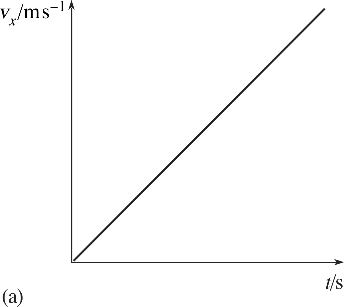
Figure 1 (a) A simple velocity–time graph.

Figure 1a shows a particularly simple velocity–time graph, that of an object released from rest at time t = 0 and falling vertically downwards with constant acceleration under the influence of gravity. As we saw in the last subsection, if we take vertically downwards to be the positive x direction then the velocity of such an object, at time t, is

v_x = gt (13)

where the constant g is the magnitude of the acceleration due to gravity. This simple relationship is reflected in the velocity–time graph where the value of v_x increases in proportion to t, i.e. it is a straight–line graph.

If we choose two particular times, t₁ and t₂ say, where t₂ > t₁, then we can see from Equation 13 (or from Figure 1b) that the corresponding values of the velocity are v_x(t₁) = gt₁ and v_x(t₂) = gt₂.

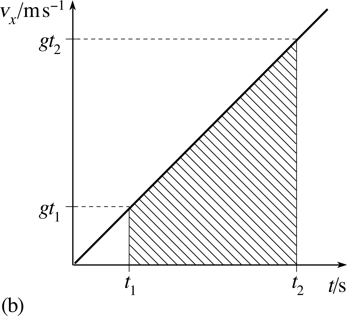
Figure 1 (b) The area under the graph between t = t₁ and t = t₂.

It follows that the average velocity of the falling object over the period from t₁ to t₂ is

½ [v_x(t₁) + v_x(t₂)] = ½ (gt₁ + gt₂)

and that the distance travelled during that time is

½ (gt₁ + gt₂)(t₂ − t₁)

Now, this distance represents the change in the position coordinate of the object over the interval t₂ − t₁ so we can write

x(t₂) − x(t₁) = ½ (gt₁ + gt₂)(t₂ − t₁)(14)

However, the right–hand side of this equation can be interpreted graphically in terms of Figure 1b as the shaded area under the velocity–time graph between t = t₁ and t = t₂. i

Note that the ‘area’ referred to here must be expressed in terms of the scale units that appear on the graph axes, not in terms of the actual area of paper in mm² or any other unit. In view of this interpretation we can say that

x(t₂) − x(t₁) = the area under the graph of v_x(t) between t₁ and t₂(15)

✦ If you take g to be 10 m s⁻², what is the hatched area in Figure 1b if t₁ = 5 s and t₂ = 10 s? What is the corresponding change in position x(t₂) − x(t₁)?

✧ The hatched area is given by

½ (50 m s⁻¹ + 100 m s⁻¹) × (10 s - 5 s) = 375 m

Consequently, x(t₂) − x(t₁) = 375 m

If we recall that x(t) is an inverse derivative of v_x(t), we can express Equation 15 in another way:

The area under the graph of v_x(t) between t = t₁ and t = t₂ is equal to the corresponding change in its inverse derivative x(t₂) − x(t₁).

Although we have only deduced this relationship for one particular form of v_x(t) it is actually a general relationship. In fact, it is a very general relationship since it not only applies to any form of v_x(t) but to any function at all, provided that function has an inverse derivative and provided we take due care over signs (see later). Subject to these provisos we can say quite generally that:

If F(x) is any one of the inverse derivatives (i.e. indefinite integrals) of f(x), then the area_under_a_grapharea under the graph of f(x), between a and b where b > a, is given by F(b) − F(a). i

In case you are worried that this result, even if true for one inverse derivative of f(x), might not be true for all the inverse derivatives of f(x), just take note of the following argument.

If F₁(x) and F₂(x) are both inverse derivatives of f(x) then we know that F₁(x) = F₂(x) + K for some constant K. It therefore follows that

F₁(b) − F₁(a) = [F₂(b) + K] − [F₂(a) + K] = F₂(b) − F₂(a)

So if the boxed result is true for one inverse derivative of f(x) it is true for any inverse derivative of f(x).

A note on notation As you can see, expressions such as F(b) − F(a) and x(t₂) − x(t₁) are very common in these discussions of inverse derivatives and the area under a graph. In order to simplify the process of writing such expressions we will henceforth indicate them by means of square brackets, as follows:

$\left[F(x)\right]_a^b = F(b) - F(a)$

and$\left[x(t)\right]_{t_1}^{t_2} = x(t) - x(t)$

The statement about the area under a graph given earlier is very important, but so far it is little more than an assertion. Before applying it to any physical or mathematical problems we should really give you a good reason for believing that it is true for any f(x).

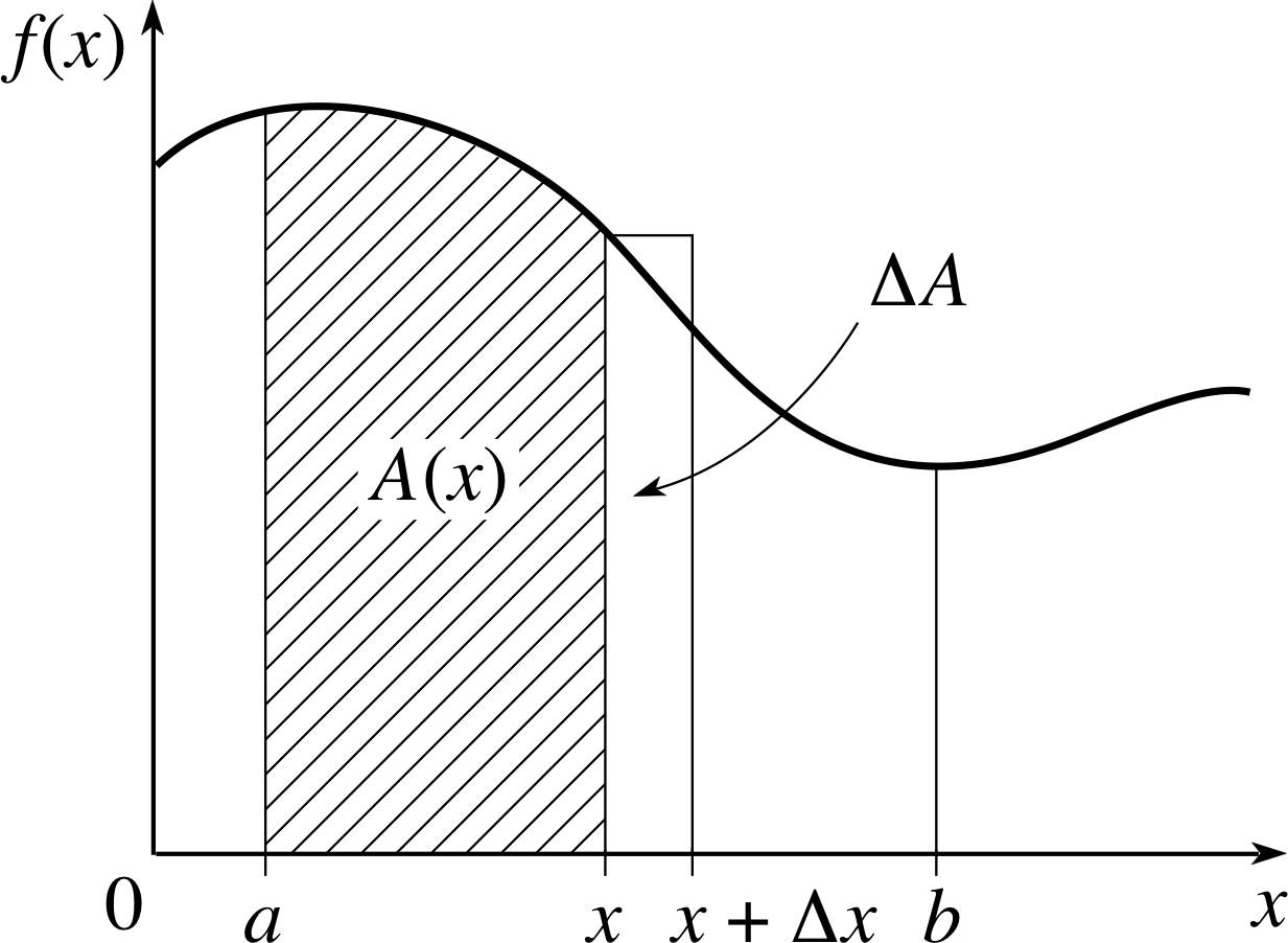
Figure 2 The graph of a general function f(x).

Figure 2 represents the graph of some general function f(x), the variable x here need not represent position, it could be any quantity. If we let a and b represent particular values of x then the shaded region in Figure 2 represents the area under the graph between x = a and some general value x that is less than or equal to b. This area (measured in the appropriate scale units) will be denoted by A(x).

If we now consider what happens to A(x) when x increases by some small amount ∆x, we can see that A(x) will also increase by an amount ∆A. We can approximate this increase in area by the area of the small rectangle shown in Figure 2, so

∆A ≈ f(x)∆x i

and therefore $\dfrac{\Delta A}{\Delta x} \approx f(x)$

Now, this approximation will become increasingly accurate as ∆x becomes smaller, so in the limit as ∆x tends to zero, we can say i

$\dfrac{dA}{dx} = f(x)$

In other words, the area function A(x) is an inverse derivative of the function f(x) whose graph has been drawn. But we have already seen that if the boxed statement is true for one inverse derivative of f(x) it is true for any inverse derivative of f(x). Since it is certainly true that the area under the graph between x = a and x = b is equal to A(b) − A(a), it follows that it is also equal to F(b) − F(a) where F(x) is any inverse derivative of f(x), as claimed.

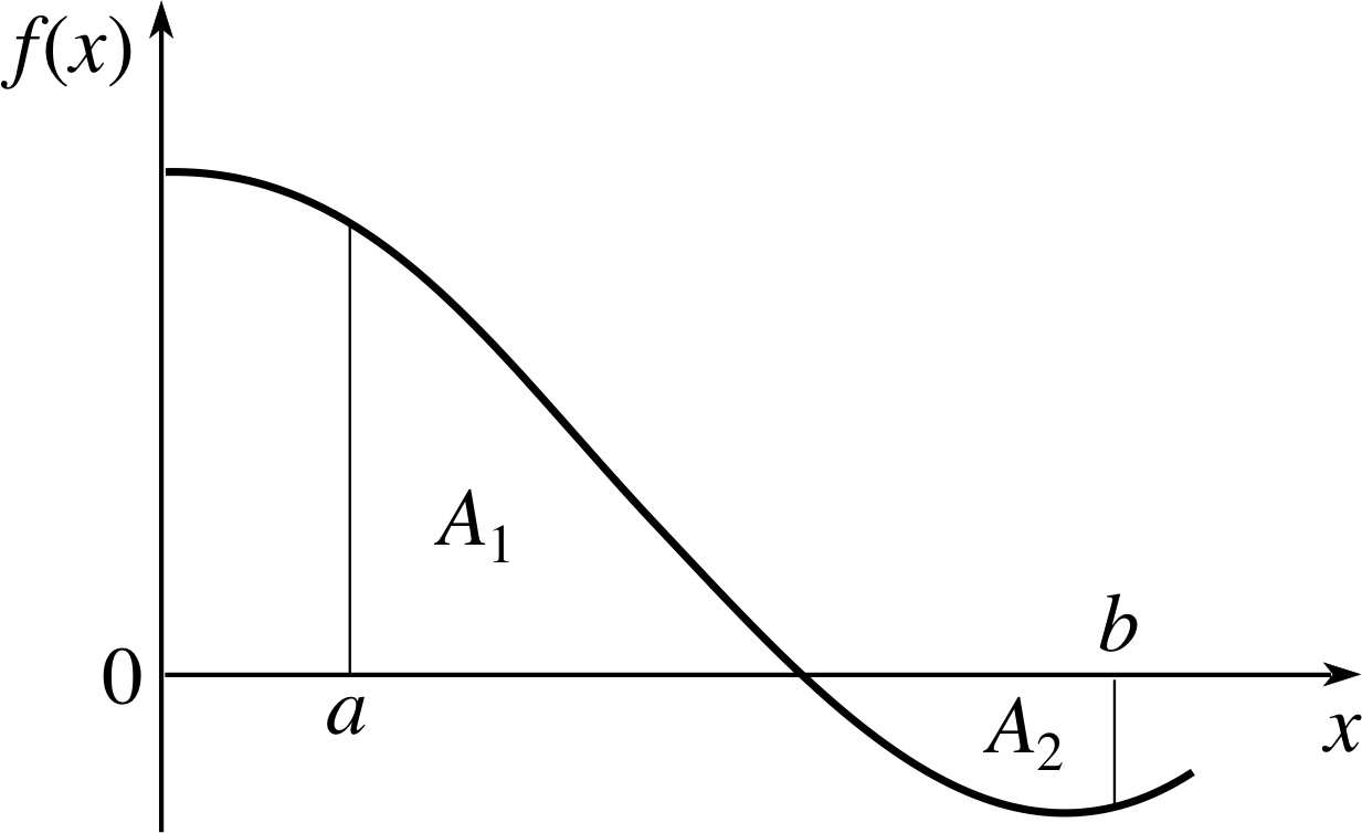
Figure 3 The area under a graph in any region where the graph is below the horizontal axis, such as A₂, will be negative. According to the convention used in FLAP, the total area under the graph in Figure 3 is A₁ + A₂ where A₂ is a negative quantity. Other authors sometimes adopt a different convention in which the area of each region is defined to be positive and the area under the graph is then given by A₁ − A₂.

Before leaving the general principles and looking at some applications, there is one more point that must be made about the area under a graph and that concerns its sign. So far, both the graphs we have considered have had the property of being positive at all points. However, as you are well aware, it is perfectly possible for a velocity v_x(t), or a general function f(x), to be negative over all or part of its domain of definition.

Would our results about inverse derivatives and areas under graphs still be true if all or part of the graph had been below the horizontal axis, as in Figure 3?

The answer is yes, though in such cases the ‘area’ below the horizontal axis (such as A₂ in Figure 3) must be treated as a negative quantity. This is a sufficiently important point that it deserves a box of its own.

When calculating the area under a graph, any regions that are below the horizontal axis should be regarded as having negative areas.

The above results can be used in two ways. If we are given, or can easily find, the area under the graph of a function, then we can determine the corresponding change in the inverse derivative. On the other hand, if we know or can easily find the inverse derivative of a function, then we can determine the area under the graph of that function. Both these applications are illustrated in the following questions which you should now attempt.

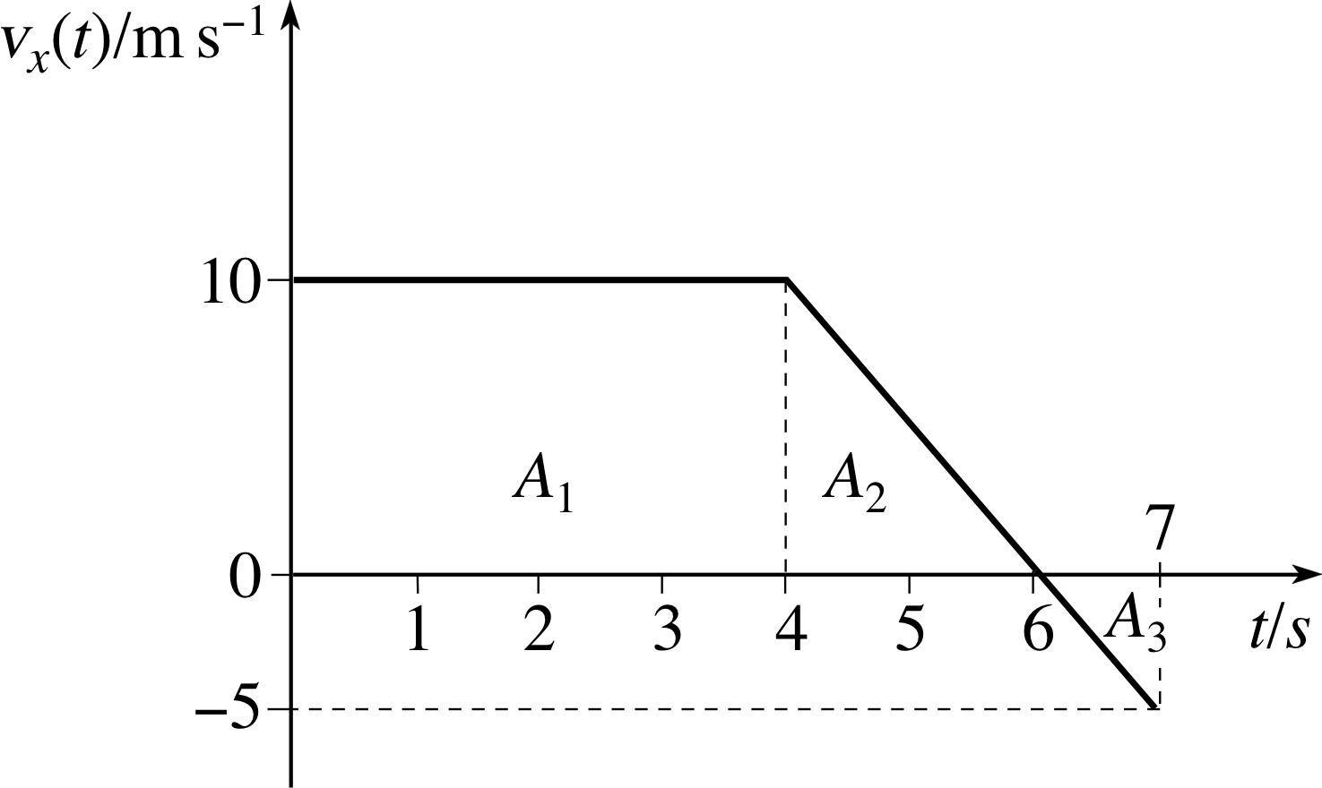
Figure 4 A velocity–time graph in which v_x(t) changes sign.

✦ Figure 4 shows the velocity–time graph of a moving object. Determine the displacement of the object from its initial position after 7 seconds. How far does the object travel during the final second of its journey? (You will need to know that the area of a triangle of base length a and height h is ½ ha.)

✧ The areas under the graph, A₁, A₂ and A₃, shown in Figure 4 are

A₁ = (10 m s⁻¹) × (4 s) = 40 m

A₂ = ½ (10 m s⁻¹) × (2 s) = 10 m

A₃ = ½ (−5 m s⁻¹) × (1 s) = −2.5 m

The displacement s_x from the initial position after 7 s is therefore

s_x(7 s) = x(7 s) − x(0) = (40 + 10 − 2.5) m − 0 m = 47.5 m

During the final second of its journey s_x changes by −2.5 m. The distance travelled during that final second is therefore 2.5 m. i

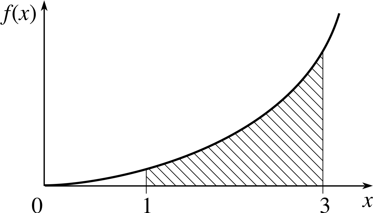
Figure 5 The graph of f(x) = 3x².

✦ Find the area under the graph of f(x) = 3x² between x = 1 and x = 3 (see Figure 5).

✧ Using inverse differentiation, we see that F(x) = x³ + C, where C is a constant, is an inverse derivative of f(x) = 3x² since $\dfrac{dF}{dx} = f(x)$.

It follows that the required area under the graph is

$\left[F(x)\right]_1^3 = \left[x^3 + C\right]_1^3 = (27 + C) - (1 + C) = 26 $

Note that in answering this last question the value of C makes no difference to the final result. Since F(x) could be any inverse derivative of f(x) it makes sense to choose the simplest and take C = 0 in such cases.

✦ Find the magnitude of the area under the graph of y = 9 − x² between x = 4 and x = 7.

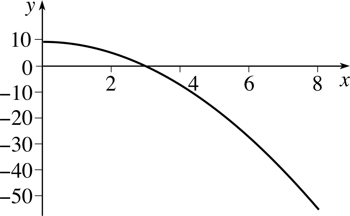
Figure 6 The graph of y = 9 − x².

✧ The graph of y = 9 − x² is shown in Figure 6.

In this case we note that an inverse derivative of y = 9 − x² is

$Y(x) = 9x - \dfrac{x^3}{3} + C$

where C is a constant.

Choosing C = 0 [WHY?], it follows that the area under the curve between x = 4 and x = 7 is

$\left[Y(x)\right]_4^7 = \left[9x - \dfrac{x^3}{3}\right]_4^7 = \left(63-\dfrac{343}{3}\right) - \left(36-\dfrac{64}{3}\right) = -66$

However, the question asks for the magnitude of the area under the curve, so the answer to the question is +66.

Question T4

(a) An object moves along a fixed x–axis at time t with velocity v_x(t) = v₀ − bt² where v₀ = 2 m s⁻¹ and b = 1 m s⁻³. Determine the displacement of the object from its initial position (i.e. its position at t = 0) after two seconds, and explain how that displacement is related to a graph of v_x against t.

(b) By noting that the velocity changes sign at t = 2 s, find the total distance travelled by the object in the first two seconds and explain how this relates to a graph of v_x against t.

Answer T4

(a) x(t) must be an inverse derivative of v_x(t), so it must be of the form

$x(t) = v_0t - b\dfrac{t^3}{3} + C$

so the required displacement is given by

$x(2\,{\rm s}) - x(0) = \left[v_0t - b\dfrac{t^3}{3} + C\right]_0^{2\,{\rm s}} = \left(2\,{\rm m\,s^{-1}}\times 2\,{\rm s} - \dfrac{1\,{\rm m\,^{-3}}\times(2\,{\rm s})^3}{3}\right) = \dfrac43\,{\rm m} \approx 1.333\,{\rm m}$

Since x(t) is one of the inverse derivatives of v_x(t), it follows that the displacement x(2 s) − x(0) is given by the area under the graph of v_x against t, between t = 0 and t = 2 s (with the areas of regions below the t–axis being treated as negative quantities).

(b) The function v_x(t) is positive for 0 ≤ t ≤ $\sqrt{2\os}$ s, so that for this time interval the displacement and the distance travelled are identical and equal to

$x(\sqrt{2\os}\,{\rm s}) - x(0) = \left[v_0t - b\dfrac{t^3}{3} + C\right]_0^{\sqrt{2\os}\,{\rm s}} = \left(2\sqrt{2\os} - \dfrac{2\sqrt{2\os}}{3}\right)\,{\rm m} = \dfrac{4\sqrt{2\os}}{3}\,{\rm m} \approx 1.886\,{\rm m}$

During the time interval $\sqrt{2\os}$ s < t ≤ 2 s the velocity is negative and the displacement is

$\begin{align} x(2\,{\rm s}) - x(\sqrt{2\os}\,{\rm s}) & = \left[v_0t - b\dfrac{t^3}{3} + C\right]_{\sqrt{2\os}\,{\rm s}}^{2\,{\rm s}} = \left(4 - \dfrac83\right)\,{\rm m} - \left(2\sqrt{2\os} - \dfrac{2\sqrt{2\os}}{3}\right)\,{\rm m}\\ & = \left(\dfrac43 - \dfrac{4\sqrt{2\os}}{3}\right)\,{\rm m} = \dfrac43\left(1- \sqrt{2\os}\right)\,{\rm m} \approx -0.552\,{\rm m}\end{align}$

However the distance travelled during this second period is given by the magnitude of the displacement, and is therefore 0.552 m. Thus, although the total displacement is 1.886 m − 0.552 m ≈ 1.33 m, the distance travelled is 1.886 m + 0.552 m ≈ 2.44 m.

In terms of a graph of v_x against t, the distance travelled is represented by the sum of the magnitudes of the areas of the various regions enclosed between the graph and the t–axis between t = 0 and t = 2 s.

2.3 Definite integrals: the limit of a sum

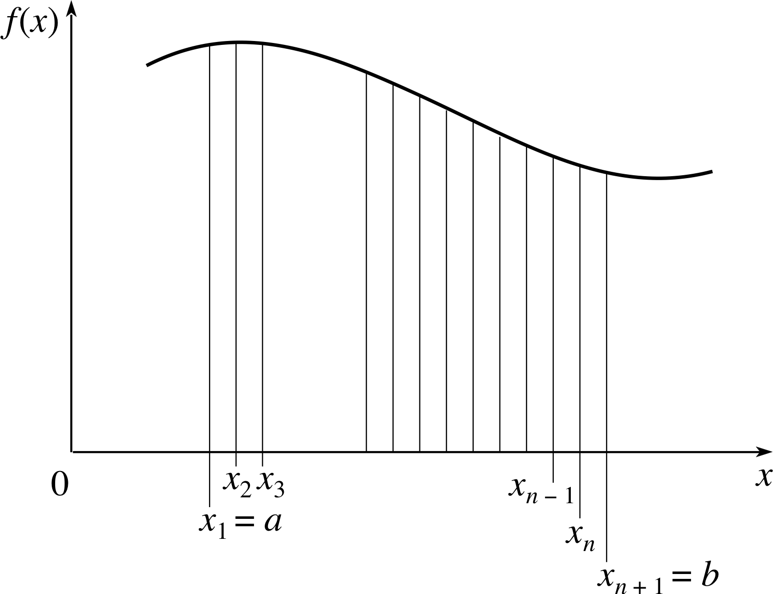
Figure 7 The area under the graph of an arbitrary function may be approximated by a sum of rectangles. (x₁ = a, x_{n + 1} = b)

We have seen how inverse differentiation can be used to find the area under the graph of a function; however there is an alternative method of evaluating areas which does not require any knowledge of inverse derivatives. This alternative technique is based on the idea that the area under a graph can be estimated by breaking it up into a large number of very thin rectangles with easily calculable areas that can be added together. This idea is illustrated in Figure 7.

In Figure 7 the area under the graph of f(x) from x₁ = a to 0 x_{n + 1} = b has been divided into n vertical strips, each of which can be approximated by rectangles. The first rectangle is of height f(x₁) and width x₂ − x₁, and the last is of height f(x_n) and width x_{n + 1} − x_n.

If we let ∆x_i = x_i+1 − x_i where i may be any whole number in the range 1 ≤ i ≤ n, i then we can say that the area of the i^th rectangle is f(x_i)∆x_i, and that the total area under the graph between a and b is approximately

$\displaystyle f(x_1)\Delta x_1 + f(x_2)\Delta x_2 + f(x_3)\Delta x_3 + \dots + f(x_n)\Delta x_n = \sum_{i=1}^nf(x_i)\Delta x_i$ i

This approximation to the area under the graph will become increasingly accurate if the number of rectangles increases and the width of the rectangles decreases. We can ensure that both requirements are met by letting ∆x denote the width of the widest rectangle, and then taking the limit of the above sum as ∆x tends to zero. Thus we have

the area under the graph of f(x) from a to b = $\displaystyle \lim_{\Delta x\rightarrow 0}\left(\sum_{i=1}^nf(x_i)\Delta x_i\right)$

Now this limit of a sum is very important, but also very cumbersome, so it is given a special name, it is called a definite integral, and it is denoted by a special symbol, a sort of distorted ‘S’ (for summation). Thus

$\displaystyle \int_a^b f(x)\,dx = \lim_{\Delta x\rightarrow 0}\left(\sum_{i=1}^nf(x_i)\Delta x_i\right)$(16)

A note on terminology Definite integrals are of such great importance that each part of the symbol has its own name. The distorted S is called an integral sign, the values a and b are known as the lower and upper limits of integration, respectively, the function that is being integrated (f(x) in this case) is called the integrand and the dx which indicates that the integration is to be performed ‘with respect to the variable x’ is called the element of integration or integration element. The use of the terms integral and integration in this context makes good sense, since they imply bringing things together to make a whole and that is exactly what a summation does.

The process of evaluating a sum and taking its limit can be very tedious, so you will be pleased to learn that there are easier ways of evaluating integrals that will be explained in the next subsection (though you might already guess what they are). However, the idea of a limit of a sum is one that arises quite naturally in many scientific problems and that is why definite integrals are an essential part of the physicist’s tool kit. In the remainder of this subsection we will show you how a finite sum can be used to estimate the value of a definite integral, and then invite you to express various physical problems in terms of definite integrals, without asking you to evaluate them.

Example 1

(a) Given that f(x) = x² + 1, write down the values of f(x) at the following values of x:

x₁ = 1.00, x₂ = 1.50, x₃ = 2.00, x₄ = 2.50, x₅ = 3.00, x₆ = 3.50 and x₇ = 4.00.

(b) By letting ∆x_i = x_i+1 − x_i, write down the value of ∆x_i for i = 1 to 6.

(c) Use your answers to (a) and (b) to work out the corresponding values of f(x_i)∆x_i and hence evaluate $\displaystyle \sum_{i=1}^6f(x_i)\Delta x_i$

(d) Explain the relationship between your answer to (c) and the definite integral ${\large\int}_1^4(x^2 + 1)\,dx$.

**Table 1** Values of f(x) = x² + 1.
i	x_i	f(x_i)	∆x_i	f(x_i)∆x_i
1	1.00	2.00	0.50	1.00
2	1.50	3.25	0.50	1.63
3	2.00	5.00	0.50	2.50
4	2.50	7.25	0.50	3.63
5	3.00	10.00	0.50	5.00
6	3.50	13.25	0.50	6.63
7	4.00	17.00
$\displaystyle \sum_{i=1}^6f(x_i)\Delta x_i = 20.39$

Solution

The answers to parts (a), (b) and (c) are given in Table 1. i

(d) The sum that has been evaluated is a crude approximation i to the given definite integral. By dividing the interval from x = 1.0 to x = 4.0 into finer parts (i.e. by using more values of x that are more narrowly separated), the quality of the approximation can be improved.

The method used to estimate the value of the definite integral in Example 1 is a crude example of a process known as numerical integration. We will not pursue that topic in this module except to note that there are far more sophisticated methods of using a finite sum to estimate the value of a definite integral, many of which can be very precise but require a great deal of repetitive labour and are therefore usually implemented on a computer.

Now try the following questions.

✦ (a) A car moves along a straight road with constant speed V for a time T = t₂ − t₁. How far does it travel in that time?

(b) At time t = t₂ the car starts to slow down, and it eventually comes to rest at time t = t₃. Throughout this period its speed is given by

v(t) = at − bt² where a and b are constants. By considering how far the car travels during a short time ∆t_i, deduce the form of

the definite integral that represents the total distance travelled between t₂ and t₃.

✧ (a) Distance travelled = VT.

(b) If the interval t₂ to t₃ is subdivided into n short intervals of duration ∆t_i then the distance travelled in any one of those intervals will be approximately

v(t_i) ∆t_i

and the total distance travelled will be approximately

$\displaystyle \sum_{i=1}^nv(t_i)\Delta t_i$

The accurate value of the total distance travelled will be given by the limit of the above sum as the number of intervals increases and the duration of the longest approaches zero, i.e. as ∆t → 0, but that is just a definite integral, so the total distance travelled between t₂ and t₃ is just

$\displaystyle \int_{t_2}^{t_3}v(t)\,dt = \int_{t_2}^{t_3}(at-bt^2)\,dt$

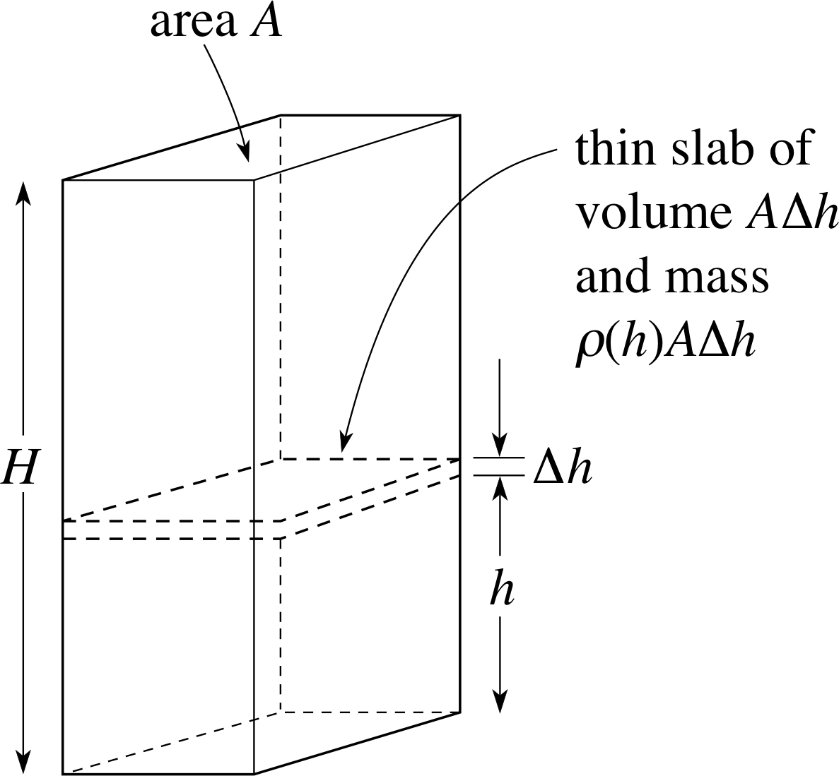
Figure 8 A column of air of height H, cross–sectional area A and variable density ρ(h).

✦ Figure 8 shows a column of atmospheric air of cross–sectional area A and total height H. At a distance h above the ground, the density of the air in the column is given by

ρ(h) = ρ₀e^−h/λ where ρ₀ and λ are constants

Use the fact that any small part of the column extending from h to h + ∆h has volume A∆h and a mass approximately given by

ρ(h)A∆h

to deduce an expression (involving a definite integral) for the total mass of the column.

✧ If the height of the column, from h = 0 to h = H, is divided into n subintervals of height ∆h_i we can approximate the mass of the column by

$\displaystyle \sum_{i=1}^n\rho(h_i)A\Delta h_i$

In the limit as the width of the largest slab tends to zero, i.e. as ∆h → 0, this sum becomes the definite integral

${\large\int}_0^H\rho(h)A\,dh = {\large\int}_0^H\rho(h){\rm e}^{-h/\lambda}\,dh$

✦ An elastic string of natural length L can be maintained at a stretched length L + x by applying a force

$F_x(x) = \dfrac{\lambda x}{L}$ where λ is a constant

In stretching the string the force is said to do work, and the work done in increasing the extension x by a small amount ∆x is approximately

F_x(x)∆x

If this approximation becomes more accurate as ∆x becomes smaller, write down a definite integral for the work done in stretching the string from its natural length to twice its natural length.

✧ The work done will be

$\displaystyle \int_0^LF_x(x)\,dx = \int_0^L\dfrac{\lambda x}{L}\,dx$ i

(Note that although the length of the string is increased from L to 2L, the extension x only increases from 0 to L, so these are the limits of integration, with respect to x, in this case.)

So much for the formulation of definite integrals by considering the limits of sums. Let us now turn to their evaluation.

2.4 The fundamental theorem of calculus

In the last subsection we were mainly concerned with the definition of a definite integral as the limit of a sum. But we started the last subsection by showing that the limit of a sum could be used to describe the area under a graph. Thus, a definite integral can be interpreted in terms of an area under a graph. However, we already know (from Subsection 2.2) that the area under the graph of a function f(x) between x = a and x = b is equal to the corresponding change in the value of its inverse derivative F(b) − F(a), where $\dfrac{dF}{dx} = f(x)$.

It follows that we can write:

If F(x) is any inverse derivative of a given function f(x), so that $\dfrac{dF}{dx} = f(x)$, then

${\Large\int}_a^bf(x)\,dx = \left[F(x)\right]_a^b = F(b) - F(a)$(17)

This remarkable result, relating the limit of a sum to a difference in inverse derivatives is known as the fundamental theorem of calculus. It provides the key to evaluating limits of sums and provides another reason for our interest in inverse derivatives. i

Example 2

Use the fundamental theorem of calculus to find the value of ${\Large \int}_1^3t^4\,dx$.

Solution

Since$\dfrac{d}{dt}\left(\dfrac{t^5}{5}\right) = t^4$

${\Large \int}_1^3t^4\,dx = \left[\dfrac{t^5}{5}\right]_1^3 = \left(\dfrac{3^5}{5}\right) - \left(\dfrac{1^5}{5}\right) = \dfrac{243}{5} - \dfrac15 = 48.4$ i

Note that the fundamental theorem applies to any inverse derivative of the integrand, so we have deliberately chosen to use the simplest in which the arbitrary constant C is zero.

✦ Use Equation 17 to evaluate the following three integrals that were obtained at the end of Subsection 2.3

(a) ${\Large \int}_{t_2}^{t_3}(at-bt^2)\,dt$, (b) ${\Large \int}_0^H\rho_0{\rm e}^{-h/\lambda}A\,dh$, (c) ${\Large \int}_0^L\dfrac{\lambda x}{L}\,dx$

✧ (a) In this case the integrand is at − bt².

An inverse derivative of this function is

$\dfrac{at^2}{2} - \dfrac{bt^3}{3} + C$ i

Choosing C = 0 [WHY?], it follows from the fundamental theorem of calculus that

$\displaystyle \int_{t_2}^{t_3}(at-bt^2)\,dt = \left[\dfrac{at^2}{2} - \dfrac{bt^3}{3}\right]_{t_2}^{t_3} = \left[\dfrac{at_3^2}{2} - \dfrac{bt_3^3}{3}\right] - \left[\dfrac{at_2^2}{2} - \dfrac{bt_2^3}{3}\right]$

i.e.$\displaystyle \int_{t_2}^{t_3}(at-bt^2)\,dt = \dfrac a2\left(t_3^2-t_2^2\right) - \dfrac b3\left(t_3^3-t_2^3\right)$

(b) In this case the integrand is Aρ₀e^−h/λ.

An inverse derivative of this function is

–Aρ₀λe^−h/λ + C.

Choosing C = 0 [WHY?], it follows from the fundamental theorem of calculus that

$\displaystyle \int_0^H\rho_0{\rm e}^{-h/\lambda}A\,dh = \left[-A\rho_0\lambda{\rm e}^{-h/\lambda}\right]_0^H = \left(-A\rho_0\lambda{\rm e}^{-H/\lambda}\right) - \left(-A\rho_0\lambda\right)$

i.e.$\displaystyle \int_0^H\rho_0{\rm e}^{-h/\lambda}A\,dh = A\rho_0\lambda(1-{\rm e}^{-H/\lambda}$

An inverse derivative of this function is

$\dfrac{\lambda x^2}{2L} + C$

Choosing C = 0 [WHY?], it follows from the fundamental theorem of calculus that

$\displaystyle \int_0^L\dfrac{\lambda x}{L} = \left[\dfrac{\lambda x^2}{2L}\right]_0^L = \dfrac{\lambda L^2}{2L} - 0 = \dfrac{\lambda L}{2}$

There are two important points to note about the answers to this question.

1: In every case the arbitrary constant C that was included in the inverse derivative played no part in the final answer since the answer only concerned a difference of the form $\left[F(x)\right]_a^b$. That is why you were able to put C = 0 in each case without any fear of error.
2: In each case the final answer only involved constants, not variables. Thus, even though we may not know the numerical values of all these constants, the result of each definite integral is itself a constant.

Question T5

Evaluate the following definite integrals.

(a) ${\Large \int}_1^2x^{1/2}\,dt$, (b) ${\Large \int}_{-2}^04x^2\,dx$, (c) ${\Large \int}_{-\pi/2}^{\pi/2}\sin x\,dx$

Answer T5

(a) ${\Large \int}_1^2x^{1/2}\,dt = \left[\dfrac{2x^{3/2}}{3}\right]_1^2 = \dfrac23\left(2^{3/2}-1\right) \approx 1.219$ since $\dfrac{d}{dx}\left(\dfrac{2x^{3/2}}{3}\right) = x^{1/2}$

(b) ${\Large \int}_{-2}^04x^2\,dx = \left[\dfrac{4x^3}{3}\right]_{-2}^0 = (0) - \left(\dfrac{-32}{3}\right) \approx 10.67$

Study comment In view of its importance it is appropriate to provide some further justification for the fundamental theorem of calculus. However such justification will not actually help you to evaluate integrals. We therefore present this justification in the form of an aside that you may regard as optional reading unless instructed otherwise by your tutor.

Aside: Justifying the fundamental theorem of calculus An informal justification for the fundamental theorem of calculus, without reference to the area under a graph, can be obtained as follows:

Since$f(x) = \dfrac{dF}{dx} = \lim_{\Delta x\rightarrow 0}\left[\dfrac{F(x+\Delta x)-F(x)}{\Delta x}\right]$

for each value of x we have

f(x)∆x ≈ F(x + ∆x) − F(x)

Now, the definite integral from a to b is obtained as the limit of a sum of terms of the form f(x_i) ∆x_i where x_i takes values

x₁, x₂, ... x_n with a = x₁ < x₂ < x₃ < ... < x_n < x_n+1 = b

and ∆x_i = x_i+1 − x_i

so that

$\begin{align} {\small\int}_a^bf(x)\,dx & \approx \sum_{i=1}^nf(x_i)\Delta x_i \approx \sum_{i=1}^n\left[F(x_{i+1}) -F(x_i)\right]\\\\[0.5em] &= \left[F(x_{n+1}) - F(x_n)\right] + \left[F(x_n) - F(x_{n-1})\right]+ \dots + \left[F(x_3) - F(x_2)\right] + \left[F(x_2) - F(x_1)\right]\end{align}$

But this last expression is equal to F(x_{n + 1}) − F(x₁), since all the intermediate terms, such as F(x_n) and F(x₂) cancel. However, x₁ = a and x_n+1 = b, so F(x_{n + 1}) − F(x₁) = F(b) − F(a).

So, in the limit we have

${\large\int}_a^bf(x)\,dx = \left[F(x)\right]_a^b = F(b) - F(a)$

thus justifying the fundamental theorem of calculus.

2.5 Indefinite integrals

Indefinite integrals are nothing new, in fact we have already remarked that ‘indefinite integral’ is an alternative term for inverse derivative; only the notation used is new.

If F(x) is an inverse derivative of f(x), so that F′(x) = f(x), then we write

${\large\int}f(x)\,dx = F(x)$, and we call ${\large\int}f(x)\,dx$ an indefinite integral of f(x). i

This is the notation and terminology that physicists generally use when dealing with inverse derivatives. All of our earlier results involving inverse derivatives can be expressed in terms of indefinite integrals and henceforth that is what we will do.

Thus, using C to represent an arbitrary constant, we can now write:

$\begin{align} & \int 3x^2\,dx = x^3 + C & &\text{since} & &\dfrac{d}{dx}(x^3+C) = 3x^2\\& \int{\rm e}^{5x}\,dx = \dfrac{{\rm e}^{5x}}{5} + C & &\text{since} & &\dfrac{d}{dx}\dfrac{{\rm e}^{5x}}{5} ={\rm e}^{5x}\\& \int\sin\left(\dfrac x2\right)\,dx = -2\cos\left(\dfrac x2\right) + C & & \text{since} & &\dfrac{d}{dx}\left[-2\cos\left(\dfrac x2\right) + C\right] = \sin\left(\dfrac x2\right)\end{align}$

In this context it clearly makes good sense to call C the constant of integration.

Notice that the indefinite integral of a function is another function. This should be contrasted with the fact that the definite integral of a function between given limits of integration is a constant.

Question T6

Find the following indefinite integrals:

(a) ${\large\int}t^3\,dt$, (b) ${\large\int}\cos x\,dx$, (c) ${\large\int}{\rm e}^{2x}\,dx$.

[Hint: Use your knowledge of differentiation to guess the answer and then check the result.]

Answer T6

(a) ${\large\int}t^3\,dt = \dfrac14t^4 + C$ since $\dfrac{d}{dx}\left(\dfrac14t^4 + C\right) = t^3$

(b) ${\large\int}\cos x\,dx = \sin x + C$ since $\dfrac{d}{dx}\left(\sin x + C\right) =\cos x$

(c) ${\large\int}{\rm e}^{2x}\,dx = \dfrac12{\rm e}^{2x} + C$ since $\dfrac{d}{dx}\left(\dfrac12{\rm e}^{2x} + C\right) = {\rm e}^{2x}$

Question T7

At time t the acceleration of an object moving along a straight line may be represented by a_x(t) = a₀(e^kt − e^−kt), where a₀ and k are constants.

(a) Evaluate ${\large\int}a_x(t)\,dt$ and explain its physical interpretation.

(b) If k = 1 s⁻¹, and if the position of the object, x(t) at time t, satisfies x(0) = 0 and x(1 s) = 1 m, find the constant of integration in ${\large\int}a_x(t)\,dt$, in terms of a₀.

Answer T7

(a) ${\Large\int}a_x(t)\,dt = \dfrac{a_0}{k}({\rm e}^{kt} + {\rm e}^{-kt}) + C$ where C is an arbitrary constant. The velocity of the moving object v_x(t) is of this form, though it includes a particular (even if unknown) value of C. Thus we can say that, apart from an additive constant, ${\large\int}a_x(t)\,dt$ represents the velocity of the moving object.

(b) From the previous part we know

$v_x(t) = \dfrac{a_0}{k}({\rm e}^{kt} + {\rm e}^{-kt}) + C$

This is a velocity. We can therefore determine

$x(t) = {\Large\int}v_x(t) = \dfrac{a_0}{k^2}({\rm e}^{kt} - {\rm e}^{-kt}) + Ct + D$

We now have two unknown constants C and D, since we have integrated twice, but we are given two pieces of

information to determine them.

First, $0 = x(0) = \dfrac{a_0}{k^2}({\rm e}^0 - {\rm e}^0) + D$ giving D = 0.

Second, since D = 0 and k = 1 s⁻¹

1 m = x(1 s) = a₀(e¹ − e⁻¹) + C

so that the required constant of integration is

$C = 1 - a_0({\rm e}^1+ {\rm e}^{-1}) = 1 - a_0\left({\rm e} - \dfrac{1}{{\rm e}}\right)$

2.6 Summary of Section 2

We now have two types of integral

(a): The definite integral: ${\large\int}_a^bf(x)\,dx$, a specific value, defined in terms of the limit of a sum and interpreted as the area under the graph of f(x) between x = a and x = b (with regions below the x–axis regarded as having negative area).
(b): The indefinite integral: ${\large\int}f(x)\,dx$, a function F(x), defined by the requirement that $\dfrac{dF}{dx} = f(x)$ and interpreted as the result of reverse differentiation. A given function f(x) generally has infinitely many indefinite integrals any two of which will differ by a constant.

These two types of integral are related by the fundamental theorem of calculus which says that if F(x) is any indefinite integral of f(x), then

${\Large\int}_a^bf(x)\,dx = \left[F(x)\right]_a^b = F(b) - F(a)$(Eqn 17)

3 The applications of integration

3.1 Some uses of integration

Integration, the analysis and evaluation of definite and indefinite integrals, is of great importance in mathematics, science and technology. We have already seen three ways in which integration can arise in physical problems:

1: as a way of reversing the effect of differentiation;
2: as a way of determining the limit of a sum;
3: as a way of determining the area under a graph (a special case of (2)).

In this subsection we look at more examples of integration to illustrate its power. It is not necessary for you to fully understand all of the physical concepts that are used in these examples in order to appreciate the mathematical points that are being made.

The mass of an object of variable density

Suppose we need to determine the mass of a solid metal bar, of length L, whose density ρ(x) at a distance x from one end is given by ρ(x) = k(x + a)² for some particular constants k and a. We suppose that the bar has a uniform square cross section of side b. The mass of the bar between x and x + ∆x is approximately b²ρ(x)∆x and the total mass is approximately obtained by adding together the masses of all these small pieces. The exact mass is given by the definite integral

${\large\int}_0^Lb^2\rho(x)\,dx = {\large\int}_0^Lkb^2(x+a)^2\,dx$

Since$\dfrac{d}{dx}\left(kb^2\dfrac{(x+a)^3}{3}\right) = kb^2(x+a)^2$ it follows that

${\large\int}_0^Lb^2\rho(x)\,dx = \left[kb^2\dfrac{(x+a)^3}{3}\right]_0^L = kb^2\dfrac{(L+a)^3}{3}-kb^2\dfrac{a^3}{3} = \dfrac{kb^2L}{3}\left(L^2+3La+3a^2\right)$

Question T8

A bar of length 2L has a circular cross section of radius R. Its density, ρ(x), i when x is measured from the mid–point of the bar, is ρ(x) = Ae^2Bx. Find an expression for the mass of the bar.

[Hint: The bar is not symmetrical.]

Answer T8

The mass of the bar between x and x + ∆x is approximately

πR²ρ(x)∆x

The exact total mass is

${\large\int}_{-L}^L\pi R^2\rho(x)\,dx$

Note that the limits are −L and L since the mi mid–point the bar is given as the origin for the density. Hence the total mass is

${\large\int}_{-L}^L\pi R^2A{\rm e}^{2Bx}\,dx = \left[\dfrac{\pi R^2}{2B}A{\rm e}^{2Bx}\right]_{-L}^L$ since $\dfrac{d}{dx}\left(\dfrac{\pi R^2}{2B}A{\rm e}^{2Bx}\right) = \pi R^2A{\rm e}^{2Bx}$

i.e.${\large\int}_{-L}^L\pi R^2A{\rm e}^{2Bx}\,dx = \dfrac{\pi R^2}{2B}A\left({\rm e}^{2BL} - {\rm e}^{-2BL}\right)$

Summing a force and calculating a total moment

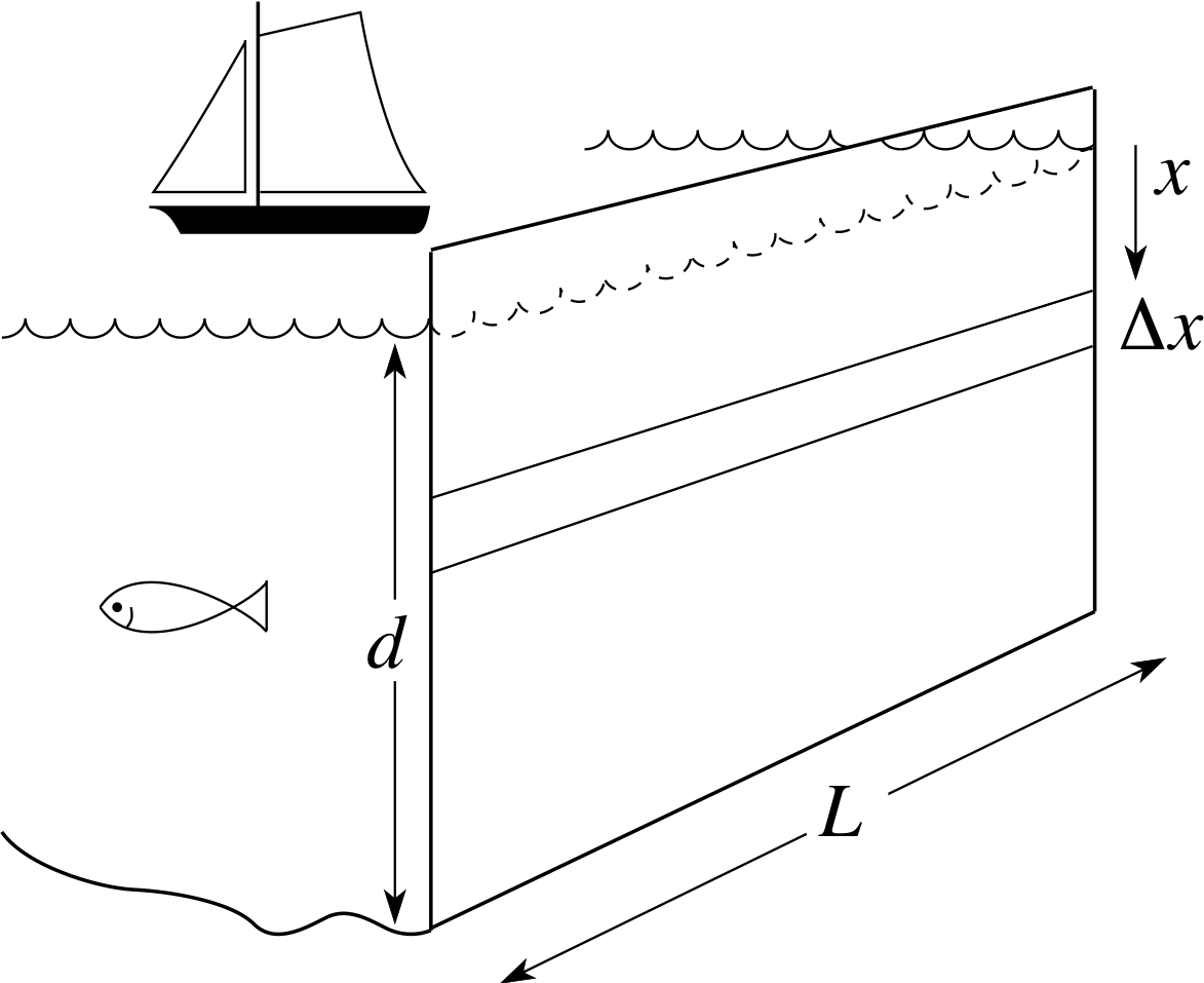
Figure 9 A rectangular dam.

Consider a simplified mathematical model of a dam in which we assume that it is rectangular in shape, of width L and depth d and placed with its plane vertical, as in Figure 9.

The pressure at a depth x below the surface of the water is P(x) = kx for some constant k, and so the magnitude of the force acting on a rectangular element of the dam wall of width L and height ∆x (and consequently area ∆A = L∆x) at a depth x is approximately

∆F ≈ P(x)∆A = Lkx∆x i

since this approximation becomes more accurate as ∆x becomes smaller, the total force on the dam is of magnitude

${\large\int}_0^dLkx\,dx = \left[\dfrac{Lkx^2}{2}\right]_0^d = \dfrac{Lkd^2}{2}$

The designers of such a dam have many other factors to take into account in addition to the total force that it must resist. For example, the pressure of the water also has a twisting effect on the structure. This twisting effect is known as the torque of the force, and for the element of area discussed above this torque about the line where the dam emerges from the water has a magnitude given by

x × Lkx∆x = Lkx²∆x

The total torque about the waterline is given by

${\large\int}_0^dLkx^2\,dx = \left[\dfrac{Lkx^3}{3}\right]_0^d = \dfrac{Lkd^3}{3}$

Finding an average

Suppose that a car completes a journey in such a way that it covers a total distance S in a time T, but at a speed v(t) that varies throughout the journey. (Remember the speed of an object is defined as the magnitude_of_a_vector_or_vector_quantitymagnitude of its velocity, so although the speed may vary it may never be negative.) Since the car covers a distance S in a time T, it is clear that its average speed is given by

$\langle v\rangle = S/T$(18) i

However, since the distance covered during any small time interval ∆t will be v(t)∆t, it is also clear that the total distance covered during the journey will be

$S = {\Large\int}_{t_1}^{t_1+T}v(t)\,dt$(19)

where t₁ denotes the time at which the journey started. It follows from Equations 18 and 19 that

$\langle v\rangle = \dfrac1T{\LARGE\int}_{t_1}^{t_1+T}v(t)\,dt$(20)

Thus, the integral provides a way of defining the average of a quantity that varies continuously. This definition has many applications.

Question T9

A bar of length 2L has a temperature T(x) that varies along its length, when x is measured from the mid–point of the bar. If Τ(x) = Acos(Bx), find an expression for the average temperature of the bar. What is the value of this average temperature if L = 2.0 m, A = 30 K and B = 0.4 m⁻¹?

Answer T9

$\langle T\rangle = \dfrac{1}{2L}{\large\int}_{-L}^LT(x)\,dx = \dfrac{1}{2L}{\large\int}_{-L}^LA\cos(Bx)\,dx = \dfrac{1}{2L}\left[\dfrac AB\sin(Bx)\right]_{-L}^L = \dfrac{1}{2L}\left[\dfrac AB\sin(Bx) + \dfrac AB\sin(Bx)\right] = \dfrac{A\sin(BL)}{L}$

Thus$\langle T\rangle = \dfrac{(30\,{\rm K})\sin(0.8)}{0.8} \approx 26.9\,{\rm K}$

3.2 The stability of a satellite

To end this section we consider one final example, concerning the stability of an orbiting satellite, that brings together some of the ideas that have been introduced earlier.

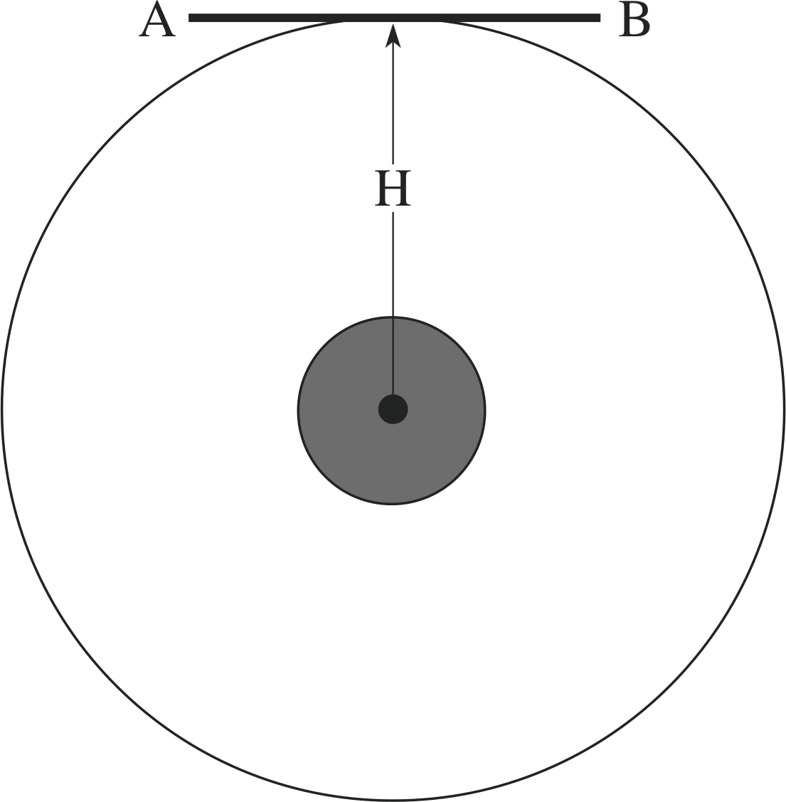
Figure 10 (a) A satellite (AB) in geostationary orbit.

The motion of a satellite in orbit about the Earth is generally very complicated, so we will consider a highly idealized case of such motion. First we will suppose that the satellite can be modelled by a uniform thin rod, of length 2L and uniform mass per unit length ρ, which means that its total mass is 2Lρ and that on the Earth’s surface it would balance about its mid–point (its centre of mass). We will also suppose that the satellite is placed in a circular geostationary orbit above the equator, in which it takes 24 hours to complete an orbit and thus appears fixed in the sky from any point on the Earth’s surface.

The distance from the centre of the Earth to the satellite will be denoted by H.

Finally, we will assume that when placed in its orbit the satellite is made to rotate about an axis through its centre at a rate of exactly 360° in 24 hours in such a way that it remains parallel to the Earth’s surface throughout its orbit (as indicated in Figure 10a). i

Once the satellite is placed in orbit (and given its initial rotation) all the stabilizers are switched off, and it is subject only to the effects of the Earth’s gravity. The question we wish to address is this: ‘Will the satellite remain with its orientation parallel to the Earth’s surface (as in Figure 10a), or will it begin to tumble?’

To answer the question we need to know a little about the force due to gravity. If two particles of mass M and m are a distance r apart, then each is attracted towards the other with a force of magnitude GmM/r² (where G is known as newtons_universal_gravitational_constantNewton’s gravitational constant).

A large spherical object, such as the Earth, exerts the same gravitational force as a particle of equal mass placed at its centre, and, since the satellite is small compared to the size of its orbit, we can assume that all the forces act vertically downwards, i.e. parallel to the line through the centre of the rod (satellite) and the centre of the Earth.

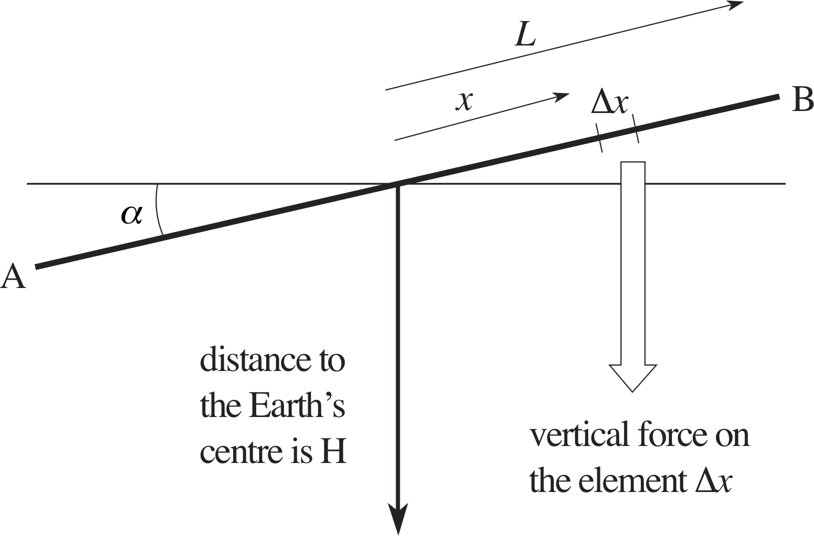
Figure 10 (b) A satellite (AB) in geostationary orbit.

We will now suppose that the satellite is disturbed very slightly, so that it is at an angle α to the horizontal (as in Figure 10b), and we will attempt to find the torque, or turning effect, of the forces due to gravity.

If we find that the torque tends to restore the satellite to its horizontal position we can conclude that the satellite is stable, but if we find that the torque tends to increase the angle α we must conclude that the satellite is unstable since a small disturbance may send it into a spin from which it will not recover.

If we consider a small element of the satellite of length ∆x with position coordinate x (measured along the satellite, from its centre), then the mass of that element will be

(density per unit length) × (length of element) = ρ∆x

and the distance of the element from the centre of the Earth will be H + xsinα.

Now the downward vertical force acting on the element will have a magnitude given approximately by

$\rm \dfrac{(gravitational~constant) \times (mass~of~Earth) \times (mass~of~element)}{(distance~of~element~from~centre~of~Earth)^2}$

So, if we represent this magnitude by ∆F and let M represent the mass of the Earth we can write

$\Delta F \approx \dfrac{GM\rho\Delta x}{(H + x\sin\alpha)^2}$

The torque, or turning effect, of the vertical force on the element, about a line that passes through the centre of the satellite and is perpendicular to the plane of Figure 10, is x∆F.

In this case ∆F (being a magnitude) must be positive, but x (and consequently x∆F) may be positive or negative. A positive torque will tend to reduce α and restore stability, a negative torque will tend to increase α and lead to instability.

To find the total torque on the satellite we need to consider the definite integral

$\displaystyle \int_{-L}^L\dfrac{GM\rho x}{(H + x\sin\alpha)^2\,dx}$

This integral can certainly be evaluated using an appropriate indefinite integral, but the techniques required to deduce that indefinite integral are beyond the scope of this module.

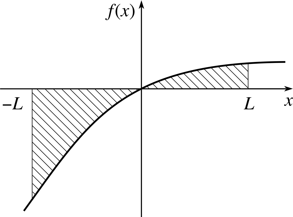
Figure 11 Areas under the graph representing the positive and negative torques acting on the satellite.

However, we can use the interpretation of a definite integral as an area under a graph to obtain the result we need. If we put

$f(x) = \dfrac{GM\rho x}{(H + x\sin\alpha)^2\,dx}$

then, for suitably chosen values of the constants, we may plot the graph of f(x), as in Figure 11.

The required integral is the area under the graph of y = f(x) between −L and L. From the graph it is easy to see that the negative contribution, from the interval −L ≤ x ≤ 0, is greater in magnitude than the positive contribution, from the interval 0 ≤ x ≤ L. This means that the net result must be negative and therefore the total moment acts so as to increase the angle α. So our conclusion is that any small disturbance of the satellite will lead to an even greater disturbance, in other words, it is unstable. i

We have only dealt with the simplest of cases. In practice one would need to consider more complicated structures, and the effects of other factors such as expansion due to solar heating, but nevertheless the example illustrates the importance of integration and the value of the methods that we have introduced in this module in evaluating physical problems.

4 Conclusion

4.1 The importance of integration

The concept of a definite integral (the limit of a sum) is fundamental to much of applicable mathematics, and is essential to a proper study of physics.

In this module we have seen how a variety of physical problems can be formulated in terms of definite integrals and we have also seen some of the ways in which such integrals can be evaluated. Finite sums and areas under graphs can both provide estimates of the values of definite integrals, but normally the most convenient method is to use the fundamental theorem of calculus to relate the definite integral to a difference in values of an appropriate indefinite integral, if such a function can be found. Almost all the definite integrals considered in this module have corresponded to indefinite integrals that it has been easy to express in terms of elementary functions (such as e^x, sinx, xⁿ, and so on). However, this is not always so. As your studies continue it is quite certain that you will encounter integrals, both definite and indefinite, of a more challenging kind. Some of the methods that can be used to deal with these integrals are explored in other FLAP modules.

The following questions are intended to improve your basic skill in evaluating integrals, and to remind you of some of the important ideas introduced in this module.

Question T10

Evaluate the following indefinite integrals:

(a) ${\large\int}(1+x+x^2)\,dx$, (b) ${\large\int}(\sin x+\cos x)\,dx$, (c)$\displaystyle \int\left({\rm e}^{-x} + \dfrac{1}{x^3}\right)\,dx$, (d) ${\large\int}2\,dw$

Answer T10

(a) ${\large\int}(1+x+x^2)\,dx = x + \dfrac{x^2}{2} +\dfrac{x^3}{3} + C$

(b) ${\large\int}(\sin x+\cos x)\,dx = \sin x - \cos x + C$

(c)$\displaystyle \int\left({\rm e}^{-x} + \dfrac{1}{x^3}\right)\,dx = -{\rm e}^{-x} - \dfrac{x^-2}{2} + C$

(d) ${\large\int}2\,dw = 2w + C$

Question T11

Evaluate the following definite integrals:

(a) $\displaystyle \int_{-1/2}^{1/2}\sin(\pi x)\,dx$, (b)$\displaystyle \int_0^3(3t+2)^2\,dt$, (c) $\displaystyle \int_0^1\dfrac{(1+{\rm e}^x)}{{\rm e}^x}\,dx$, (d) $\displaystyle \int_1^4\sqrt{x\os}(x+1)\,dx$.

Answer T11

(a) $\displaystyle \int_{-1/2}^{1/2}\sin(\pi x)\,dx = \left[-\dfrac{\cos(\pi x)}{\pi}\right]_{-1/2}^{1/2} = 0$

You see why this must be zero just by sketching a graph of y = sin(πx).

(b)${\Large\int}_0^3(3t+2)^2\,dt = {\Large\int}_0^3(9t^2+12t+4)\,dt = \left[3t^3+6t^2+4t\right]_0^3 = 147$

(c) $\displaystyle \int_0^1\dfrac{(1+{\rm e}^x)}{{\rm e}^x}\,dx = \int_0^1({\rm e}^{-x}+1)\,dx = \left[-{\rm e}^{-x}+x\right]_0^1 = \left(-\dfrac{1}{{\rm e}}+1\right) - (-1) = 2 - \dfrac{1}{{\rm e}}$

(d) ${\Large\int}_1^4\sqrt{x\os}(x+1)\,dx ={\Large\int}_1^4(x^{3/2}+x^{1/2})\,dx = \left[\dfrac{2x^{5/2}}{5} + \dfrac{2x^{3/2}}{3}\right] = \dfrac{256}{15} \approx 17.067$

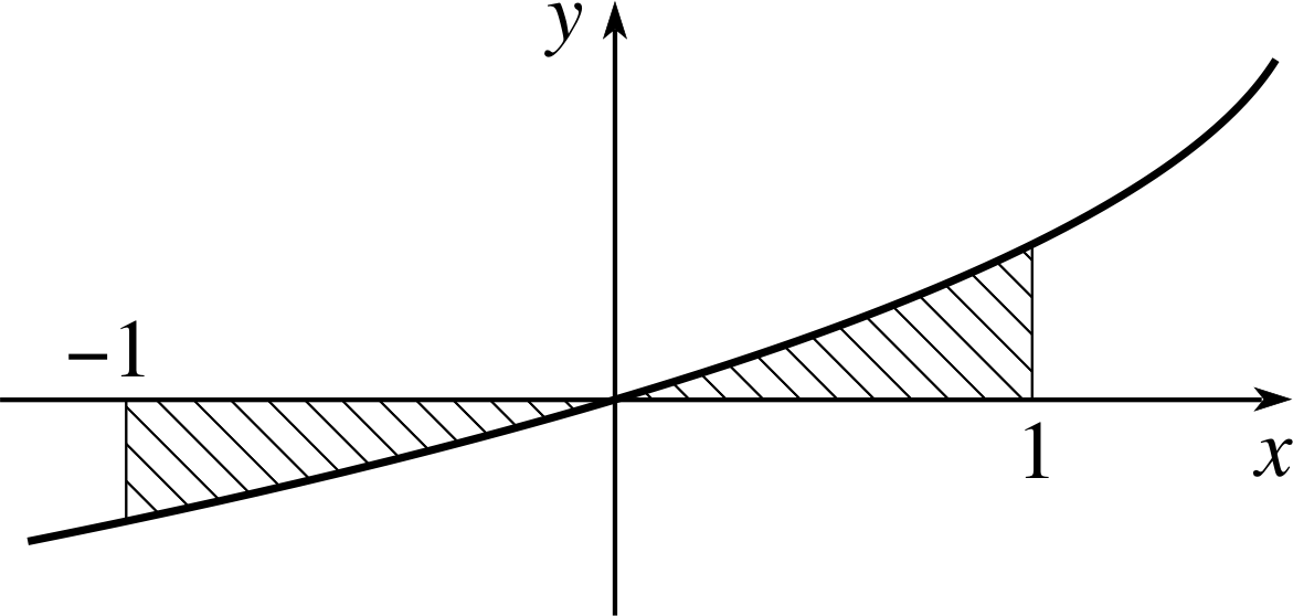
Figure 12 See Question T12.

Question T12

Find the sum of the magnitudes of the two shaded areas in Figure 12, i.e. find the magnitude of the area enclosed by the graph of the function y = e^x − 1, the x–axis and the lines x = −1 and x = 1. Note that in this case you are not being asked for ‘the area under the graph’ which may be negative, but for the magnitude of the area enclosed, which must be positive.

Answer T12

We must evaluate the area in two parts, since the graph lies below the x–axis for −1 ≤ x < 0 and above the x–axis for 0 < x ≤ 1 (see Figure 12).

${\Large\int}_{-1}^0({\rm e}^x-1)\,dx = \left[{\rm e}^x-x\right]_{-1}^0 = 1 - \left[{\rm e}^{-1}-(-1)\right] = -\dfrac{1}{\rm e}$

and${\Large\int}_0^1({\rm e}^x-1)\,dx = \left[{\rm e}^x-x\right]_0^1 = ({\rm e} - 1) - 1= {\rm e} - 2$

In FLAP we would normally say that these answers represented the areas under the graph in the two regions, even though one of them is a negative quantity because it lies below the horizontal axis. However, in this problem we are specifically asked for the magnitudes of the areas enclosed, so the required answer is

$\lvert\,{\rm e} - 2\,\rvert + \left\lvert\, - \dfrac{1}{\rm e}\,\right\rvert = {\rm e} + \dfrac{1}{\rm e} - 2$

Question T13

The acceleration, velocity and position coordinate of an object moving along a straight line are represented by a_x(t), v_x(t) and x(t), respectively. What physical meaning, if any, can you associate with the following?

$\displaystyle \int_{t_1}^{t_2}a_x(t)\,dt$, $\displaystyle \int_{t_1}^{t_2}v_x(t)\,dt$, $\displaystyle \int_{t_1}^{t_2}x(t)\,dt$

Answer T13

${\Large\int}_{t_1}^{t_2}a_x(t)\,dt$ represents the area under the graph of a_x(t) against t between the points t = t₁ and t = t₂, assuming that areas above the t–axis are assigned a positive value and areas below the t–axis are assigned a negative value. Physically, it represents the change in the velocity of the object from time t₁ to time t₂.

${\Large\int}_{t_1}^{t_2}v_x(t)\,dt$ represents the area under the graph of v_x(t) against t between the points t = t₁ and t = t₂, assuming that areas above the t–axis are assigned a positive value and areas below the t–axis are assigned a negative value. Physically, it represents the change in the position of the object from time t₁ to time t₂.

${\Large\int}_{t_1}^{t_2}x(t)\,dt$ represents the area under the graph of x(t) against t between the points t = t₁ and t = t₂, assuming that areas above the t–axis are assigned a positive value and areas below the t–axis are assigned a negative value. There is no other particular physical significance for this integral.

5 Closing items

5.1 Module summary

1

If f(x) is a given function and F(x) is any function such that $\dfrac{dF}{dx} = f(x)$ then we write $F(x) = {\large\int}f(x)\,dx$ and we call F(x) an Subsection 2.5indefinite integral (or Subsection 2.5inverse derivative or Subsection 2.5primitive) of f(x).

2

If F₁(x) and F₂(x) are both indefinite integrals of the same function f(x), then there exists a constant K such that

F₁(x) = F₂(x) + K

3

For motion in a straight line, if the position, velocity and acceleration at time t are respectively x(t), v_x(t) and a_x(t) then

$v_x(t) = \dfrac{dx}{dt}\quad\text{and}\quad a_x(t) = \dfrac{dv_x}{dx}$

so,$x(t) = {\large\int}v_x(t)\,dt\quad\text{and}\quad v(t) = {\large\int}a_x(t)\,dt$

4

The Subsection 2.3definite integral of a function f(x) from x = a to x = b is defined by the limit of a sum and may be written as

$\displaystyle \int_a^b f(x)\,dx = \lim_{\Delta x\rightarrow 0}\left(\sum_{i=1}^nf(x_i)\Delta x_i\right)$(Eqn 16)

where ∆x is the width of the largest subinterval, and where x₁ = a and x_n+1 = b.

5

According to the Subsection 2.4fundamental theorem of calculus, if F(x) is any indefinite integral of a given function f(x), so that $\dfrac{dF}{dx} = f(x)$, then

${\Large\int}_a^bf(x)\,dx = \left[F(x)\right]_a^b = F(b) - F(a)$(Eqn 17)

This often provides a convenient way of evaluating definite integrals.

6

The definite integral ${\Large\int}_a^bf(x)\,dx$, with b > a, may be interpreted as the area under the graph of f(x) between x = a and x = b. i It follows from the fundamental theorem of calculus that the area under the graph of f(x) between x = a and x = b is equal to the corresponding change in the indefinite integral, F(b) − F(a). When calculating the area under a graph, any regions that are below the horizontal axis should be regarded as having negative areas.

5.2 Achievements

Having completed this module, you should be able to:

A1: Define the terms that are emboldened and flagged in the margins of the module.
A2: Define an indefinite integral of a given function in terms of a process that reverses the effect of differentiation, and use that definition to express physical quantities (such as position and velocity, in the case of linear motion) as indefinite integrals of other physical quantities (such as velocity and acceleration).
A3: Determine (by inspection) indefinite integrals of a range of simple functions in various mathematical and physical contexts, recognizing that the process of indefinite integration generally introduces an arbitrary constant.
A4: Define the definite integral of a given function between given limits in terms of the limit of a sum, and use that definition to formulate various physical problems in terms of definite integrals.
A5: Recognize that the definition of a definite integral as the limit of a sum can be used to justify the use of a finite sum to estimate the value of a given definite integral.
A6: Interpret the definite integral of a given function between given limits in terms of the area under the graph of that function between those limits (with due regard to signs), and use this identification to determine areas and/or evaluate definite integrals in sufficiently simple cases.
A7: State the fundamental theorem of calculus that relates definite and indefinite integrals, and use it to evaluate definite integrals in sufficiently simple cases.

Study comment You may now wish to take the following Exit test for this module which tests these Achievements. If you prefer to study the module further before taking this test then return to the topModule contents to review some of the topics.

5.3 Exit test

Study comment Having completed this module, you should be able to answer the following questions, each of which tests one or more of the Achievements.

Question E1 (A2, A3 and A5)

The acceleration of an object moving along the x–axis is given at time t by

a_x(t) = a₀(e^t/k + e^−t/k)

where a₀ and k are constants. If a₀ = 2.00 m s⁻² and k = 1.00 s, obtain expressions for the velocity v_x(t) and the position x(t) given that v_x(0) = x(0) = 0.

What is the area under the graph of a_x(t) against t between t = 1 s and t = 2 s, and what does this area represent?

Answer E1

Given that a_x(t) = a₀(e^t/k + e^−t/k) we have v_x(t) = a₀k(e^t/k − e^−t/k) + C

Since v_x(0) = 0 it follows that C = 0, and therefore x(t) = a₀k²(e^t/k + e−^t/k) + D

We are told that x(0) = 0 so that 0 = a₀k²(1+ 1) + D and therefore D = −2a₀k² (which implies D = −4), and it follows that x(t) = a₀k²(e^t/k + e^−t/k − 2)

The area under the graph of a_x(t) between t = 1 s and t = 2 s is given by

${\large\int}_{1\,{\rm s}}^{2\,{\rm s}}a_x(t) = v_x(2\,{\rm s}) - v_x(1\,{\rm s}) = a_0k\left[{\rm e}^{t/k} - {\rm e}^{-t/k}\right]_{1\,{\rm s}}^{2\,{\rm s}}$

i.e.${\large\int}_{1\,{\rm s}}^{2\,{\rm s}}a_x(t) = (2.00\,{\rm m\,s^{-1}}) - v_x(1\,{\rm s}) = \left[({\rm e}^2 - {\rm e}^{-2}) - ({\rm e}^1 - {\rm e}^{-1})\right] \approx 9.81\,{\rm m\,s^{-1}}$

This area represents the change in the velocity over this time interval.

(Reread Subsection 2.1Subsections 2.1, Subsection 2.22.2 and Subsection 2.32.3 if you had difficulty with this question.)

Question E2 (A5 and A6)

The indefinite integral ${\large\int}\exp(x^2)\,dx$ i cannot be expressed in terms of elementary functions, so it is not possible to evaluate the definite integral ${\large\int}_0^1\exp(x^2)\,dx$ in a straightforward way using the fundamental theorem of calculus. Describe two other ways in which you might estimate the value of this definite integral. (You are not required to perform these evaluations.)

**Table 2** A crude numerical integration.
i	x_i	f(x_i) = exp(x_i²)	f(x_i)∆x_i
1	0.0	1.0000	0.100 00
2	0.1	1.0101	0.101 01
3	0.2	1.0408	0.104 08
4	0.3	1.0942	0.109 42
5	0.4	1.1735	0.117 35
6	0.5	1.2840	0.128 40
7	0.6	1.4333	0.143 33
8	0.7	1.6323	0.163 23
9	0.8	1.8965	0.189 65
10	0.9	2.2479	0.224 79
Approximation for ${\large\int}_0^1f(x)\,dx = 1.381 26$

Answer E2

One way to find an approximation for ${\large\int}_0^1\exp(x^2)\,dx$ is to let f(x) = exp(x²) and divide the interval from x = 0 to x = 1 into n subintervals, each of length ∆x_i. The sum ${\large\sum}_{i=1}^nf(x_i)\Delta x_i$ (evaluating the function at the left–hand end of each subinterval say) then provides a numerical estimate of the definite integral. The result of doing this with ten equal subintervals is shown in Table 2.

This is a crude form of numerical integration, more sophisticated methods give 1.462 65 as a better estimate.

Another method of estimating the value of the integral is to draw the graph of the function and then measure the area under that graph between the given limits. If you were to adopt this method you would have to remember to quote the measured area in terms of the scale units used on the graph’s axes.

(Reread Subsection 2.2Subsections 2.2 and Subsection 2.32.3 if you had difficulty with this question.)

Question E3 (A3)

Evaluate the following indefinite integrals.

(a) ${\large\int}x^{1/2}\,dx$, (b) ${\large\int}(x+3)(x+2)\,dx$, (c) ${\large\int}6\cos(3x)\,dx$, (d) ${\large\int}({\rm e}^x + {\rm e}^{-x})({\rm e}^x - {\rm e}^{-x})\,dx$.

[Hint: By expanding where appropriate, you should be able to determine by inspection (i.e. guess) a function which, when differentiated, produces the given integrand in each case.]

Answer E3

In the following solutions, C is an arbitrary constant.

(a) ${\large\int}x^{1/2}\,dx = \dfrac23x^{3/2} + C$ since $\dfrac{d}{dx}\left(\dfrac23x^{3/2} + C\right) = x^{1/2}$

(b) ${\large\int}(x+3)(x+2)\,dx = {\large\int}(x^2+5x+6)\,dx = \dfrac13x^3 + \dfrac52x^2 + 6x + C$

since$\dfrac{d}{dx}\left(\dfrac13x^3 + \dfrac52x^2 + 6x + C\right) = x^2 + 5x +6$

(d) ${\large\int}({\rm e}^x + {\rm e}^{-x})({\rm e}^x - {\rm e}^{-x})\,dx = {\large\int}({\rm e}^{2x} + {\rm e}^{-2x})\,dx = \dfrac12{\rm e}^{2x} + \dfrac12{\rm e}^{-2x} + C$

since$\dfrac{d}{dx}\left(\dfrac12{\rm e}^{2x} + \dfrac12{\rm e}^{-2x} + C\right) = {\rm e}^{2x} + {\rm e}^{-2x}$

(Reread Subsection 2.1Subsections 2.1 and Subsection 2.52.5 if you had difficulty with this question.)

Question E4 (A7)

Use the fundamental theorem of calculus to evaluate each of the integrals in Question E3

(a) ${\large\int}x^{1/2}\,dx$, (b) ${\large\int}(x+3)(x+2)\,dx$, (c) ${\large\int}6\cos(3x)\,dx$, (d) ${\large\int}({\rm e}^x + {\rm e}^{-x})({\rm e}^x - {\rm e}^{-x})\,dx$

between 0 and 1, i.e. with lower limit 0 and upper limit 1.

Answer E4

In each of the following solutions we will not include the arbitrary constant since it cancels when calculating each definite integral.

(a) ${\large\int}_0^1x^{1/2}\,dx = \left[\frac23x^{3/2}\right]_0^1 = \frac23- 0 = \frac23$

(b) ${\large\int}_0^1(x+3)(x+2)\,dx = \left[\frac13x^3 + \frac52x^2 + 6x\right]_0^1 = \left(\frac13 + \frac52 + 6\right) - \left(0\vphantom{\frac00}\right) \approx 8.83$

(d) ${\large\int}_0^1({\rm e}^x + {\rm e}^{-x})({\rm e}^x - {\rm e}^{-x})\,dx = \left[\frac12{\rm e}^{2x} + \frac12{\rm e}^{-2x}\right]_0^1 = \frac12({\rm e}^2 + {\rm e}^{-2}) - \frac12({\rm e}^0 + {\rm e}^0) = \frac12({\rm e}^2 + {\rm e}^{-2}) - 1 \approx 2.762$

(since e⁰ = 1)

(Reread Subsection 2.3 if you had difficulty with this question.)

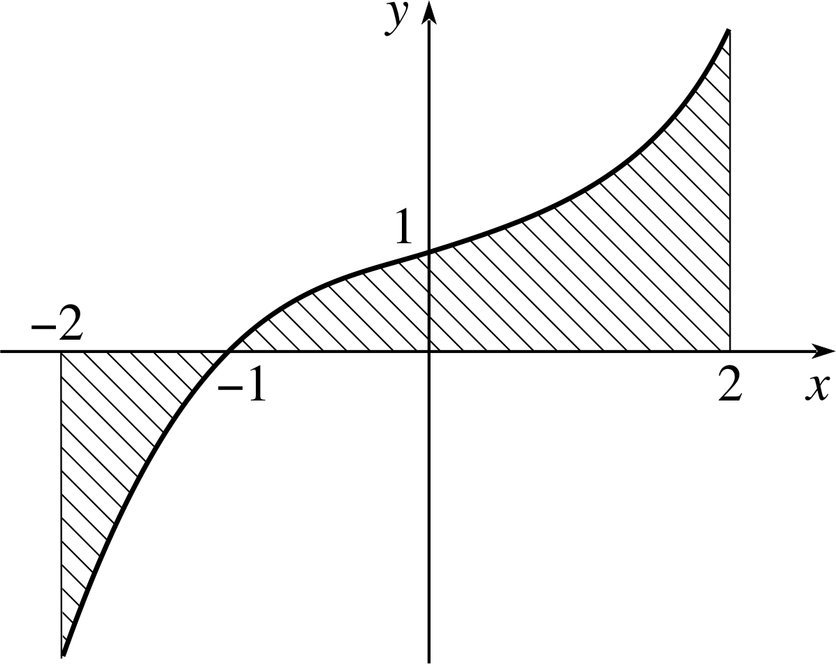
Figure 13 See Question E5.

Question E5 (A3, A6 and A7)

Find the sum of the magnitudes of the shaded areas in Figure 13, i.e. find the area enclosed by the graph of the function y = x³ + 1, the x–axis and the lines x = −2 and x = 2.

(Note that in this case you are not being asked for ‘the area under the graph,’ which would be the difference of these magnitudes.)

Answer E5

The required area is calculated in two parts: first the portion between x = −2 and x = −1, second, the portion between x = −1 and x = 2. The first part is

${\Large\int}_{-2}^{-1}\left(x^3+1\right)\,dx = \left[\frac14x^4+x\right]_{-2}^{-1} = \left(\frac14-1\right) - \left(\frac14\times 16-2\right) = -\frac34- 2 = -2.75$

So the magnitude of the area is 2.75. The second part is

${\Large\int}_{-1}^2\left(x^3+1\right)\,dx = \left[\frac14x^4+x\right]_{-1}^2 = \left(\frac14\times 16+2\right) - \left(\frac14- 1\right) = 6 + \frac34 = 6.75$

The required answer is therefore, 2.75 + 6.75 = 9.5.

(Reread Subsection 2.2Subsections 2.2, Subsection 2.32.3 and Subsection 2.42.4 if you had difficulty with this question.)

Study comment This is the final Exit test question. When you have completed the Exit test go back and try the Subsection 1.2Fast track questions if you have not already done so.

If you have completed both the Fast track questions and the Exit test, then you have finished the module and may leave it here.

MATH 5.1: Introducing integration

PPLATO / FLAP (Flexible Learning Approach To Physics)

MATH 5.1: Introducing integration

1 Opening items

1.1 Module introduction

1.2 Fast track questions

1.3 Ready to study?

2 The concept of integration

2.1 Inverse derivatives: reversing differentiation

2.2 Inverse derivatives and the area under a graph

2.3 Definite integrals: the limit of a sum

2.4 The fundamental theorem of calculus

2.5 Indefinite integrals

2.6 Summary of Section 2

3 The applications of integration

3.1 Uses of integration

3.2 The stability of a satellite

4 Conclusion

4.1 The importance of integration

5 Closing items

5.1 Module summary

5.2 Achievements

5.3 Exit test

1 Opening items

1.1 Module introduction

1.2 Fast track questions

1.3 Ready to study?

2 The concept of integration

2.1 Inverse derivatives: reversing differentiation

Motion with uniform acceleration under gravity

Motion with non–uniform acceleration

2.2 Inverse derivatives and the area under a graph

2.3 Definite integrals: the limit of a sum

Example 1

Solution

2.4 The fundamental theorem of calculus

Example 2

Solution

2.5 Indefinite integrals

2.6 Summary of Section 2

3 The applications of integration

3.1 Some uses of integration

The mass of an object of variable density

Summing a force and calculating a total moment

Finding an average

3.2 The stability of a satellite

4 Conclusion

4.1 The importance of integration

5 Closing items

5.1 Module summary

5.2 Achievements

5.3 Exit test

FLAP material © copyright 1996 Open University