MATH 4.5: Taylor expansions and polynomial approximations |
PPLATO @ | |||||
PPLATO / FLAP (Flexible Learning Approach To Physics) |
||||||
|
1 Opening items
1.1 Module introduction
Many of the functions used in physics (including sin(x), tan(x) and loge(x)) are impossible to evaluate exactly for all values of their arguments. In this module we study a particular way of representing such functions by means of simpler polynomial functions of the form a0 + a1x + a2x2 + a2x3 ..., where a0, a1, a2, etc. are constants, the values of which depend on the function being represented. Sums of terms of this kind are generally referred to as series. The particular series we will be concerned with are known as Taylor series. We also show how, in certain circumstances, the first few terms of a Taylor series can give a useful approximation to the corresponding function.
For a physicist, the ability to find Taylor approximations is arguably the most useful skill in the whole ‘mathematical tool-kit’. It allows many complicated problems to be simplified and makes some mathematical models easier to solve and, perhaps more important, easier to understand.
Section 2 of this module begins by showing how some common functions can be approximated by polynomials. In each case the polynomial has the property that the values of its low–order derivatives, when evaluated at a particular point, are the same as those of the function which it approximates.
In Section 3 we show how this feature leads to a general technique for representing functions by means of series, and how taking the first few terms of such series can provide a useful approximation to the corresponding function. Subsection 3.1Subsections 3.1 and Subsection 3.23.2 are concerned with Taylor polynomials and series where the argument, x, of the corresponding function is close to zero. In Subsection 3.3Subsections 3.3 and Subsection 3.43.4 we consider polynomials and series for which x is not close to zero. Subsection 3.6 gives some useful tricks and short–cuts which can be used when finding Taylor polynomials and series. Subsection 3.5 lists some standard Taylor series, and Subsection 3.7 gives some applications of the ideas introduced in this module.
Study comment Having read the introduction you may feel that you are already familiar with the material covered by this module and that you do not need to study it. If so, try the following Fast track question. If not, proceed directly to the Ready to study? in Subsection 1.3.
1.2 Fast track questions
Study comment Can you answer the following Fast track questions? If you answer the questions successfully you need only glance through the module before looking at the Subsection 4.1Module summary and the Subsection 4.2Achievements. If you are sure that you can meet each of these achievements, try the Subsection 4.3Exit test. If you have difficulty with only one or two of the questions you should follow the guidance given in the answers and read the relevant parts of the module. However, if you have difficulty with more than two of the Exit questions you are strongly advised to study the whole module.
Question F1
Write down the general expression for the Taylor expansion of a function, f (x), about the point x = a. Use this series to find the first five terms in the expansion of $\sqrt{x^\os}$ about x = 1. i
Answer F1
The Taylor series for f (x) near x = a is
$f(x) = f(a) + f'(a)(x-a) + \dfrac{f''(a)}{2!}(x-a)^2 + \dfrac{f^{(3)}(a)}{3!}(x-a)^3 + \dots + \dfrac{f^{(n)}(a)}{n!}(x-a)^n + \dots$
It is implicit that the derivatives, f (n)(a) (for n ≥ 0), all exist.
If we write $f(x) = \sqrt{x}$ then
$\begin{align} f(1) & = \left[x^{1/2}\right]_{x=1} = 1\\ f'(1) & = \left[\dfrac{1}{2}x^{-1/2}\right]_{x=1} = \dfrac{1}{2}\\ f''(1) & = \left[\left(\dfrac{1}{2}\right)\left(\dfrac{-1}{2}\right)x^{-3/2}\right]_{x=1} = \left(\dfrac{1}{2}\right)\left(\dfrac{-1}{2}\right)\\ f^{(3)}(1) & = \left[\left(\dfrac{1}{2}\right)\left(\dfrac{-1}{2}\right)\left(\dfrac{-3}{2}\right)x^{-5/2}\right]_{x=1} = \left(\dfrac{1}{2}\right)\left(\dfrac{-1}{2}\right)\left(\dfrac{-3}{2}\right)\end{align}$
In general we have
$f^{(n)} = \underbrace{\left(\dfrac{1}{2}\right)\left(\dfrac{-1}{2}\right)\left(\dfrac{-3}{2}\right)\left(\dfrac{-5}{2}\right)\dots}_{\color{purple}{\large{n~\text{terms}}}}$
and therefore
$\begin{align} x^{1/2} & = 1 + \dfrac{(x-1)}{2} + \dfrac{1}{2}\left(\dfrac{-1}{2}\right)\dfrac{(x-1)^2}{2!} + \dfrac{1}{2}\left(\dfrac{-1}{2}\right)\left(\dfrac{-3}{2}\right)\dfrac{(x-1)^3}{3!} + \dfrac{1}{2}\left(\dfrac{-1}{2}\right)\left(\dfrac{-3}{2}\right)\left(\dfrac{-5}{2}\right)\dfrac{(x-1)^4}{4!} + \dots\\ & = 1 + \dfrac{(x-1)}{2} - \dfrac{(x-1)^2}{8} + \dfrac{(x-1)^3}{16} - \dfrac{5(x-1)^4}{128}\dots\end{align}$
Question F2
Write down the Taylor expansions of exp(x) and sin(x) about x = 0, and hence find the first three non–zero terms in the Taylor expansion of exp(x2) sin(2x) about x = 0.
Answer F2
We have$\exp(x) = 1 + x + \dfrac{x^2}{2!} + \dots$
and$\sin(x) = x - \dfrac{x^3}{3!} + \dfrac{x^5}{5!} - \dots$
so that$\exp(x^2)\sin(2x) = \left[1 + x^2 + \dfrac{x^4}{2!} + \dots\right]\times\left[(2x) - \dfrac{(2x)^3}{3!} + \dfrac{(2x)^5}{5!} - \dots\right]$
and, expanding the brackets, the right–hand side becomes:
$2x + \left(2-\dfrac{2^3}{3!}\right)x^3 + \left(\dfrac{2}{2!}-\dfrac{2^3}{3!} + \dfrac{2^5}{5!}\right)x^5 + \dots = 2x + \dfrac{2}{3}x^3 - \dfrac{1}{15}x^5 + \dots$
1.3 Ready to study?
Study comment To begin the study of this module you need to be familiar with the following terms: approximation (≈), constant, factorial (n!), function, gradient (of a graph), modulus (or absolute value, e.g. | x |), power_mathematicalpower, radian, root_of_an_equationroot, summation symbol (∑), tangent_to_a_curvetangent (to a curve) and variable. You should also be familiar with the following topics: sketching graphs of elementary functions (such as y = sin(x)); finding nth order derivatives of simple functions; the properties (including derivatives and values at important points) of the elementary functions, such as the trigonometric_functionstrigonometric, exponential_functionsexponential and logarithmic_functionslogarithmic functions, simplifysimplifying, expand_an_expressionexpanding and calculationevaluating algebraic expressions. Some familiarity with infinite series and the convergent_seriesconvergence of such series would also be useful, but this is not essential. If you are unfamiliar with any of these topics, you should consult the Glossary, which will indicate where in FLAP they are developed. The following Ready to study questions will help you to establish whether you need to review some of the above topics before embarking on this module.
Question R1
Find the value of the derivative of 1 + 2x + 3x2 at x = 2.
Answer R1
$\dfrac{d}{dx}(1 + 2x + 3x^2) = 2 + 6x = 14$ when x = 2.
Consult differentiation in the Glossary for further details.
Question R2
What are the values of n! for n = 0, 1, 2, 3, 4?
Answer R2
The factorial function is defined by
0! = 1 and n! = n × (n − 1)! for n ≥ 1
so we have
0! = 1, 1! = 1, 2! = 2, 3! = 3 × 2 × 1 = 6
and4! = 4 × 3 × 2 × 1 = 24
Consult factorial in the Glossary for further information.
Question R3
Simplify the following expression
$\displaystyle \sum_{n=0}^{n=4}2^nx^n - \sum_{n=0}^{n=3}x^n$
and give your answer without using the summation symbol.
Answer R3
$\displaystyle \sum_{n=0}^{n=4}2^nx^n - \sum_{n=0}^{n=3}x^n = (1+2x+4x^2+8x^3+16x^4)-(1+x+x^2+x^3) = x+3x^2+7x^3+16x^4$
Consult summation in the Glossary for further information.
Question R4
Using primes to denote differentiation, find f (1), f ′ (1), f ′′ (1) and f (3)(1) for
f (x) = x3 + x4
Answer R4
$f(1) = [x^3+x^4]_{x=1} = 2$
$\begin{align} f'(1) & = \left[\dfrac{df}{dx}\right]_{x=1} & = \left[3x^2+4x^3\right]_{x=1} & = 7\\ f''(1) & = \left[\dfrac{d^2f}{dx^2}\right]_{x=1} & = \left[6x+12x^2\right]_{x=1} & = 18\\ f^{(3)}(1) & = \left[\dfrac{d^3f}{dx^3}\right]_{x=1} & = \left[6+24x\os\right]_{x=1} & = 30\end{align}$
Consult derivatives and order_of_a_derivativenth order derivatives in the Glossary for further information.
Question R5
If p (x) is defined by
p (x) = 1 + 3x + 2x2
write down simplified expressions for p (−x), p (2x) and p (1 + 2x).
Answer R5
p (−x) = 1 + 3 (−x) + 2 (−x)2 = 1 − 3x + 2x2
p (2x) = 1 + 3 (2x) + 2 (2x)2 = 1 + 6x + 8x2
p (1 + 2x) = 1 + 3 (1 + 2x) + 2 (1 + 2x)2 = 1 + 3 (1 + 2x) + 2 (1 + 4x + 4x2)
p (1 + 2x) = (1 + 3 + 2) + x (6 + 8) + 8x2 = 6 + 14x + 8x2
Consult simplifysimplifying equations in the Glossary for further information.
Question R6
Given that P (x) = 1 + x + x2 and Q (x) = 2 − x + 3x2, expand and simplify P (x)Q (x).
Answer R6
P (x)Q (x) = (1 + x + x2)(2 − x + 3x2) = 2 + x + 4x2 + 2x3 + 3x4
Consult expand_an_expressionexpanding expressions in the Glossary for further information.
2 Polynomial approximations
2.1 Polynomials
Many different kinds of functions are used throughout mathematics and physics. Whereas some functions, such as
$f(x) = x - \dfrac{x^3}{6} + \dfrac{x^5}{120}$(1)
$g(x) = 1 + \dfrac{x}{2} - \dfrac{x^2}{8}$(2)
h (x) = 1 + x(3)
are polynomial functions, others, such as
u (x) = sin(x)(4)
$v(x) = \sqrt{1 + x^{\phantom 0}}$(5)
$w(x) = \dfrac{1}{1-x}$(6)
are not.
A function p (x) is a polynomial function of x (or in x) if it can be expressed in the form
p (x) = a0 + a1x + a2x2 + a3x3 + ... + anx n(7)
in other words, as a sum of powers of x, with each power multiplied by a coefficient (a0, a1, and so on). The powers of x are non–negative integers.
While it is easy to see that expressions such as 1 + 2x − x2 − x3 and x5 + (x − 1)4 are polynomials in x, it is not always so easy. For example,
(ex − e−x)2 − (ex + e−x)2 + (x sin x)2 + (x cos x)2
is actually a polynomial in x (in fact −4 + x2), but it may take a few moments thought to see why this is so.
✦ Which of the following are polynomials in x?
(a) 1 + x + (x − 1)2, (b) 1 + ex + e2x, (c) $\dfrac{1}{1+x+x^2}$, (d) $1 + \dfrac{1}{x} + \dfrac{1}{x^2} + \dfrac{1}{x}^3$.
✧ Only (a) is a polynomial in x.
The highest power of the variable in a polynomial is known as the degree_of_a_polynomialdegree of the polynomial. For example, in the above expression for p (x) (Equation 7) the degree is n (assuming that an is non-zero).
Question T1
What are the degrees of the polynomial functions f (x), g (x) and h (x), defined in Equations 1, 2 and 3?
$f(x) = x - \dfrac{x^3}{6} + \dfrac{x^5}{120}$(Eqn 1)
$g(x) = 1 + \dfrac{x}{2} - \dfrac{x^2}{8}$(Eqn 2)
h (x) = 1 + x(Eqn 3)
Answer T1
f (x), g (x) and h (x) are of degree 5, 2 and 1, respectively.
Low-order polynomials are often given special names. Polynomials of degree zero are simply constants; polynomials of degree one are called linear; those of degree two are called quadratic and those of degree three are called cubic_functioncubic. i
An important property of any polynomial, p (x), is that for any value of x, the value of p (x) can be calculated by simply using the arithmetic operations of addition (or subtraction) and multiplication. This is not the case with many other functions (for example, u (x), v (x) and w (x), defined in Equations 4, 5 and 6)
u (x) = sin(x)(Eqn 4)
$v(x) = \sqrt{1 + x^{\phantom 0}}$(Eqn 5)
$w(x) = \dfrac{1}{1-x}$(Eqn 6)
and it can be very useful to know polynomial approximations to such functions.
Question T2
Plot the functions h (x) and w (x) (defined in Equations 3 and 6)
h (x) = 1 + x(Eqn 3)
$w(x) = \dfrac{1}{1-x}$(Eqn 6)
on the same graph for 0 ≤ x ≤ 0.9. Compare the two curves. [Hint: You do not need to plot these functions ‘by hand’. If you have access to a graph plotting calculator or computer program, use it!]
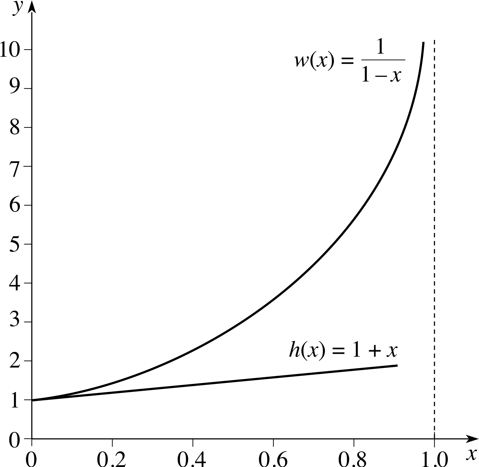
Figure 9 See Answer T2.
Answer T2
The functions h (x) = 1 + x and w (x) = 1/(1 − x) are sketched in Figure 9. We can see that the two graphs are approximately the same for small values of x, but that the difference between the two becomes progressively larger as x increases.
The exercise that you have just completed shows that, for y ‘small’ values of x, the polynomial function h (x) is approximately the same as w (x), so here we have an example of a polynomial approximation to the function 1/(1 − x).
However, we can see from Figure 9 that the approximation becomes progressively worse as x increases towards the value 1.
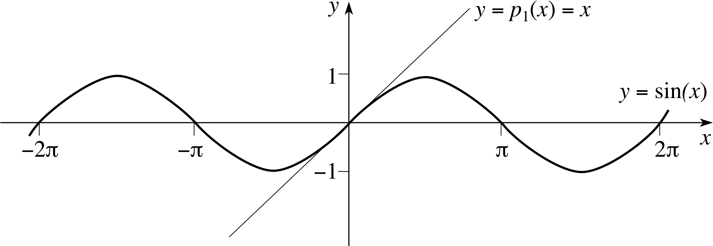
Figure 1 Graphs of the functions y = x and y = sin(x). Note that throughout this module the argument of any trigonometric function is either a dimensionless variable or an angle in radians rather than degrees.
In Figure 1 we have plotted the graphs of y = sin(x) and y = x on the same axes.
As you can see, the graphs of the two functions are very similar for small values of | x |, i but as | x | increases, the discrepancy gets progressively worse, so that for | x | above about 0.7 it is very noticeable, and above π/2 (i.e. approximately 1.57) the two graphs show no similarity at all.

Figure 2 A simple pendulum.
So there may be circumstances where we would be justified in approximating sin(x) by x, but such an approximation is only likely to be useful for small values of | x |.
For example, an analysis of the motion of a simple pendulum gives the (apparently intractable) equation
$\dfrac{d^2}{dt^2}[\theta(t)] = -\omega^2\sin[\theta(t)]$(8) i
where θ (t) is the angle shown in Figure 2 and ω is a constant (called the angular frequency). For small deviations of the pendulum from the vertical, θ (t) is small, and we are justified in making the approximation sin(θ) ≈ θ, giving
$\dfrac{d^2}{dt^2}[\theta(t)] = -\omega^2\theta(t)$
which is straightforward to solve.
Question T3
Show that θ (t) = sin(ωt) is a solution of
$\dfrac{d^2}{dt^2}[\theta(t)] = -\omega^2\theta(t)$(9)
but not of
$\dfrac{d^2}{dt^2}[\theta(t)] = -\omega^2\sin[\theta(t)]$(Eqn 8)
Answer T3
We have $\dfrac{d}{dt}\sin(\omega t) = \omega\cos(\omega t)$ and $\dfrac{d}{dt}\cos(\omega t) = -\omega \sin(\omega t)$
and therefore $\dfrac{d^2}{dt^2}\theta(t) = \dfrac{d^2}{dt^2}\sin(\omega t) = \omega\dfrac{d}{dt}\cos(\omega t) = -\omega^2 \sin(\omega t) = \omega^2\theta(t)$
which shows that θ (t) = sin(ωt) is a solution of
$\dfrac{d^2}{dt^2}\theta(t) = \omega^2\theta(t)$
On the other hand, if we try θ (t) = sin(ωt) as a solution of
$\dfrac{d^2}{dt^2}\theta(t) = \omega^2\sin[\theta(t)]$
we find that the left–hand side is −ω2sin(ωt) (as before) but the right–hand side is now −ω2sin[sin(ωt)], and these two functions of t are certainly not equal.
2.2 Increasingly accurate approximations for sin(x)
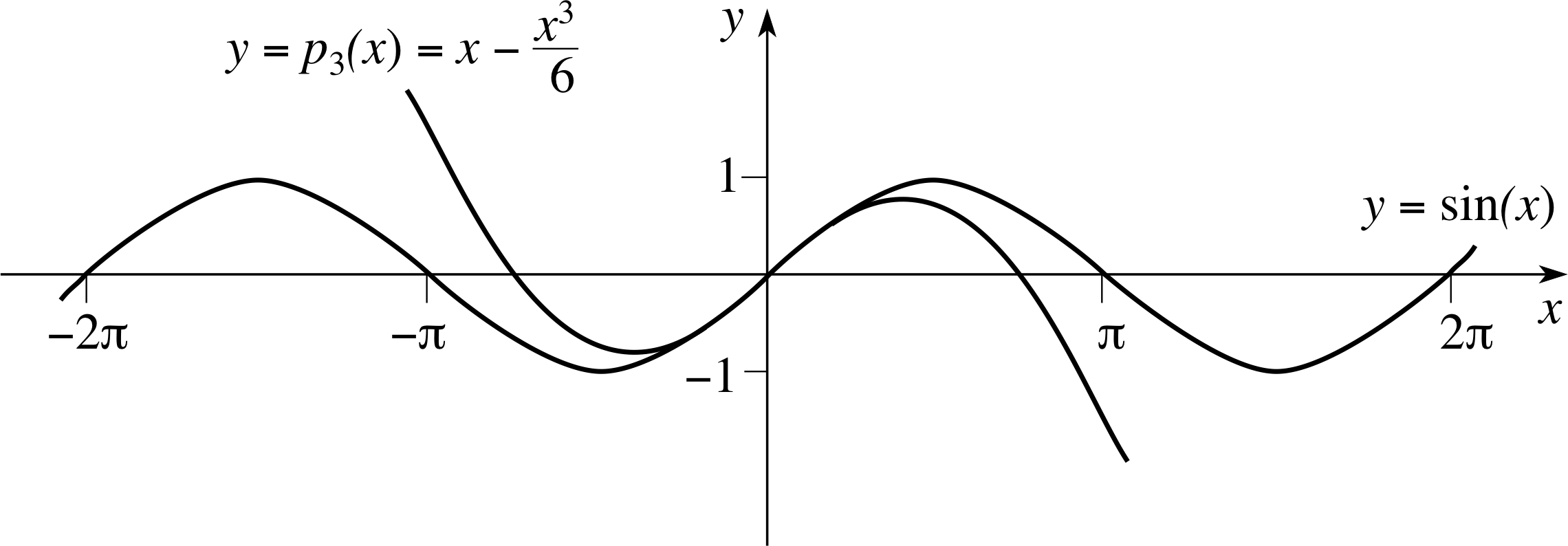
Figure 3 Graphs of the functions y = x − (x3/6) and y = sin(x).
If we put
p1(x) = x(10)
then our previous discussion amounts to saying that p1(x) is an acceptable approximation for sin(x) provided that | x | is small.
However, for many applications, particularly those involving ‘large’ values of x, approximating sin(x) by p1(x) is not at all satisfactory.
Fortunately there are better approximations. For example, in Figure 3 we plot the polynomial
$p_3(x) = x - \dfrac{x^3}{6}$(11) i
together with the sin(x) function.
If you compare Figure 3 with Figure 1, you can see that this polynomial is a much better approximation to the sine function than the linear polynomial and is particularly good for | x | less than about 1.5.
✦ How is this new approximation p3(x) related to the previous approximation p1(x)?
✧ The coefficient of x in the two expressions is identical. In other words the approximation is improved by adding an extra term and not by changing the existing one.
You may be wondering how we were able to choose a polynomial p3(x) that works so well.
The answer lies in a comparison of the derivatives of sin(x) and p3(x) at x = 0, as follows, where for convenience we have written f (x) = sin(x), and we use primes (′) to indicate differentiation.
| The function f (x) = sin(x), at x = 0 i |
The approximating polynomial p3(x) = x − (x3/6) at x = 0 |
|---|---|
| f (0) = sin(0) = 0 | $p_3(0)=\left[x-\dfrac{x^3}{6}\right]_{x=0} = 0$ |
| f ′ (0) = cos(0) = 1 | $p'_3(0)=\left[1-\dfrac{x^2}{2}\right]_{x=0} = 1$ |
| f ′′ (0) = −sin(0) = 0 | $p''_3(0)=\left[-x\right]_{x=0} = 0$ |
| f (3)(0) = −cos(0) = −1 | $p^{(3)}_3(0) = -1$ |
For convenience we also introduce the notation [ ]x=0 to indicate that the function inside the brackets should be evaluated at the value outside.
As you can see, the values of the functions sin(x) and p3(x), and their first three derivatives, are precisely the same when evaluated at x = 0.
By using higher–degree polynomials it is possible to obtain increasingly accurate approximations to sin(x). For example,
$p_5(x) = x - \dfrac{x^3}{6} + \dfrac{x^5}{120}$(12)
is a polynomial approximation of degree five to sin(x), which gives very accurate results near x = 0. Shortly we will show you how we found p5(x), but first, to see how good this new approximation really is, try the following question.
Question T4
Find p5(0.2) as accurately as you can, and compare your answer to that obtained for sin(0.2) on a calculator.
Answer T4
$p_5(x) = x - \dfrac{x^3}{6} + \dfrac{x^5}{120} = 0.2 - 3\times 10 + 15\times 10 \approx 0.198\,669\,333\,333$
My calculator gives the answer sin(0.2) = 0.198 669 330 795, so the approximating polynomial gives the correct answer to eight decimal places.
| The function f (x) = sin(x), at x = 0 |
The approximating polynomial (Equation 12) at x = 0 |
|---|---|
| f (0) = sin(0) = 0 | $p_5(0)=\left[x-\dfrac{x^3}{6}+\dfrac{x^5}{120}\right]_{x=0} = 0$ |
| f ′ (0) = cos(0) = 1 | $p'_5(0)=\left[1-\dfrac{x^2}{2}+\dfrac{x^4}{24}\right]_{x=0} = 1$ |
| f ′′ (0) = −sin(0) = 0 | $p''_5(0)=\left[-x+\dfrac{x^3}{6}\right]_{x=0} = 0$ |
| f (3)(0) = −cos(0) = −1 | $p^{(3)}_5(0) = \left[-1+\dfrac{x^2}{2}\right]_{x=0} = -1$ |
| f (4)(0) = sin(0) = 0 | $p^{(4)}_5(0) = \left[x\right]_{x=0} = 0$ |
| f (5)(0) = cos(0) = 1 | $p^{(5)}_5(0) = 1$ |
The polynomial p5(x) was chosen so that its value, and the values of its first five derivatives, at x = 0, are the same as for sin(x). i We can see that this is the case by performing a calculation similar to that which we performed for p3(x).
✦ How is this new approximation, p5(x), for sin(x) related to the previous approximation p3(x)?
✧ The coefficients of x and x3 in the two expressions are identical. So once again the approximation is improved by leaving the existing terms unchanged, and adding an extra term.
The previous discussion suggests that we may be able to construct a sequence of increasingly accurate approximations to sin(x):
$p_1(x) = x,~~p^3(x) = x - \dfrac{x^3}{6},~~p^5(x) = x - \dfrac{x^3}{6} + \dfrac{x^5}{120}$, and so on
which are obtained by adding higher and higher powers of x.
So far we have verified that these polynomials and their derivatives behave very like sin(x) at x = 0, but we have not shown you how to construct them. We will remedy this deficiency shortly, but first let us try a similar idea on a function other than sin(x).
2.3 Increasingly accurate approximations for exp(x)
Since exp(0) = e0 = 1, it is clear that exp(x) i is approximately equal to 1 when x is close to 0 but perhaps we can find a better approximation.
We could try a polynomial which is linear in x, that is
q1(x) = a0 + a1x(13)
and look for numbers, a0 and a1, such that the low–order derivatives of exp(x) and q1(x) are identical.
| The function g (x) = exp(x), at x = 0 |
The approximating polynomial (Equation 13) at x = 0 |
|---|---|
| g (0) = exp(0) = 0 | $q_1(0)=\left[a_0 + a_1x\right]_{x=0} = a_0$ |
| g ′ (0) = exp(0) = 1 | $q'_1(0)=\left[a_1\right]_{x=0} = a_1$ |
Remembering that $\dfrac{d}{dx}[\exp(x)] = \exp(x)$, and writing g (x) = exp(x) for convenience, we can construct the table on the right.
So, if we choose a0 = 1 and a1 = 1, the approximating polynomial becomes
q1(x) = 1 + x
and its value, and the value of its first derivative are, respectively, identical to the values of exp(x) and its first derivative at x = 0.
✦ Evaluate q1(0.1) and exp(0.1). What is the gradient of y = exp(x) at x = 0? What is the equation of the tangent to the graph of y = exp(x) at x = 0?
✧ q1(0.1) = 1.1 and exp(0.1) ≈ 1.105 1709, so q1(x) is a good approximation to exp(x) at x = 0.1.
The gradient of y = exp(x) is
$\dfrac{dy}{dx} = \exp(x)$.
So at x = 0 the gradient is exp(0) = 1.
The tangent line at x = 0 has the equation y = 1 + x (and this is why q1(x) = 1 + x is a good approximation to exp(x) near x = 0).
| The function g (x) = exp(x), at x = 0 |
The approximating polynomial q2(x) = a0 + a1x + a2x2 at x = 0 |
|---|---|
| g (0) = exp(0) = 0 | $q_2(0)=\left[a_0 + a_1x + 2_2x^2\right]_{x=0} = a_0$ |
| g ′ (0) = exp(0) = 1 | $q'_2(0)=\left[a_1+2a_2x\right]_{x=0} = a_1$ |
| g ′′ (0) = exp(0) = 1 | $q''_2(0)=\left[2a_2\right]_{x=0} = 2a_2$ |
Now let us try to find a better approximation by considering a quadratic polynomial
q2(x) = a0 + a1x + a2x2
and look for numbers, a0, a1, a2, such that the low–order derivatives of exp(x) and q2(x) are identical. Constructing a table of values as before, we have the table to the right.
So if we match the functions and their derivatives at x = 0 by choosing a0 = 1, a1 = 1 and 2a2 = 1 the approximating polynomial becomes
$q_2(x) = 1 + x + \dfrac{x^2}{2}$(14)
✦ Using Equation 14, compare q2(0.1) with q1(0.1) and exp(0.1).
✧ q2(0.1) = 1.105 which is a better approximation to exp(0.1) ≈ 1.105 1709 than q1(0.1) = 1.1.
Once again we have obtained a better approximation by adding a term of higher degree, x2/2 in this case, while the constant term and the coefficient of x remain unchanged. As you might imagine, we can continue this process by considering the cubic polynomial
q3(x) = a0 + a1x + a2x2 + a3x3(15)
and arranging that the low–order derivatives of exp(x) and q3(x) are identical.
✦ Calculate a3 and hence find q3(x).
✧ If g (x) = exp(x) then g(3)(0) = exp(0) = 1 while q3(3)(0) = 3 × 2 × a3 = 6a3 and these derivatives are equal if 6a3 = 1, and therefore i
$q_3(x) = 1 + x + \dfrac{x^2}{2} + \dfrac{x^3}{6}$(16)
✦ Compare q3(0.1) with q1(0.1), q2(0.1) and exp(0.1).
✧ q3(0.1) = 1.105 166 67 which is a better approximation to exp(0.1) ≈ 1.105 1709 than q2(0.1) = 1.105 and q1(0.1) = 1.1.
Question T5
Use your calculator to obtain exp(x) and q3(x) (to three decimal places) for x = 0, 0.1, 0.5, 1.0, 2, 10. What conclusions can you draw from comparing the two sets of results?
| x | exp(x) | q3(x) |
|---|---|---|
| 0 | 1.0 | 1.0 |
| 0.1 | 1.105 | 1.105 |
| 0.5 | 1.649 | 1.646 |
| 1.0 | 2.718 | 2.667 |
| 2.0 | 7.389 | 6.333 |
| 10.0 | 22 026.466 | 227.667 |
Answer T5
The values are given in Table 2.
From these results we can see that for small values of x, q3(x) is a very good approximation to exp(x). But as x increases the approximation gets progressively worse, with the error always having the same sign. For x = 10, the approximation is useless.
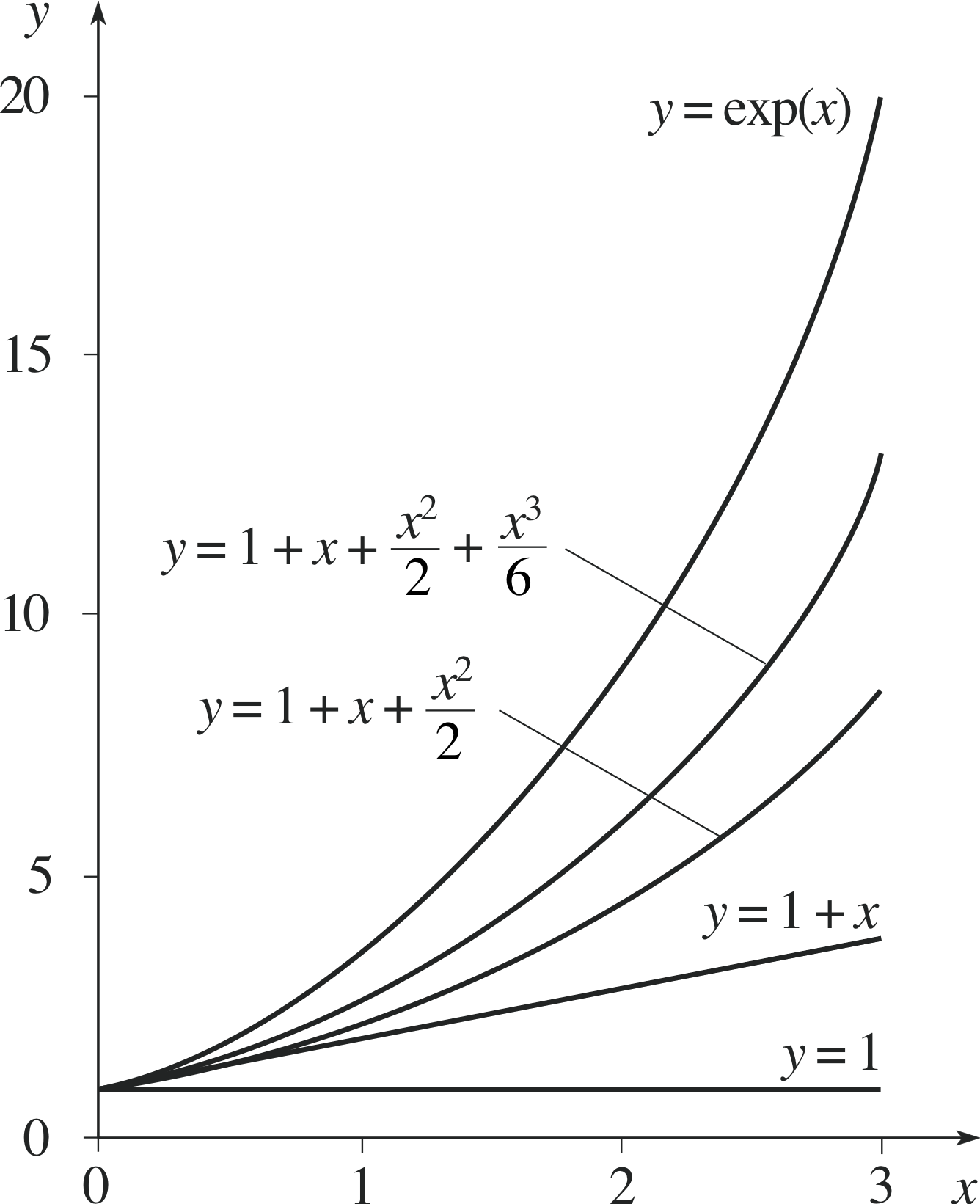
Figure 4 Polynomial approximations to exp(x).
Some conclusions
So it appears that the polynomials
$1,~1+x,~1+x+\dfrac{x}{2},~1+x+\dfrac{x}{2}+\dfrac{x^3}{6}$, and so on
provide a sequence of increasingly accurate approximations to exp(x) for small values of x, and in particular for exp(0.1). In each case a better approximation is obtained by adding a term with a higher power of x, and choosing the coefficient so that the low–order derivatives of the polynomial and exp(x) are identical at x = 0.
Sketching exp(x) and these polynomials for a range of values of x, as in Figure 4, suggests that the polynomials also provide increasingly accurate approximations for other values of x. Our aim in the next section is to generalize this technique for finding polynomial approximations.
3 Finding polynomial approximations by Taylor expansions i
3.1 Taylor polynomials (near x = 0)
So far, we have considered polynomial approximations to the sine and exponential functions, but in this subsection we intend to apply a similar method to approximate the general function f (x) near to x = 0 by a polynomial
pn(x) = a0 + a1x + a2x2 + a3x3 + ... + anx n(17)
where n ≥ 0 indicates the degree of the approximating polynomial.
The purpose of this subsection is to show you how to choose the coefficients (i.e. the numbers a0, a1, a2 and so on); but first try the following preliminary exercises.
Preliminary exercises
✦ Given that p (x) = 1 + 3x + 5x2 + 7x3 + 9x4 write down expressions for p ′ (x), p ′′ (x) and p ′′ (0).
✧ p ′ (x) = 3 + 10x + 21x2 + 36x3, p ′′ (x) = 10 + 42x + 108x2 and p ′′ (0) = 10. i
✦ Elsewhere in this subsection pn(x) refers to the general polynomial defined by Equation 17,
pn(x) = a0 + a1x + a2x2 + a3x3 + ... + anx n(Eqn 17)
but suppose for the purposes of this question that pn(x) is the particular polynomial defined by
$p_n(x) = 1 + \dfrac{x}{1.1}+\dfrac{x^2}{1.2}+\dfrac{x^3}{1.3}+\cdots+\dfrac{x^n}{(1+n\times 0.1)}$
(a) what are the coefficients a0, a3, a10 and an?
(b) Write down expressions for pn′ (x) and pn′′ (x).
(c) What is the value of pn′′ (0)?
✧ (a) a0 = 1, a3 = 1/(1.3), a10 = 1/2 and an = 1/(1 + n × 0.1).
(b) $p'_n(x) = \dfrac{1}{1.1} + \dfrac{2x}{1.2} + \dfrac{3x^2}{1.3} + \cdots + \dfrac{nx^{n-1}}{(1+n\times 0.1)}$ and $p''_n(x) = \dfrac{2}{1.2} + \dfrac{3x2\times x}{1.3} + \cdots + \dfrac{n(n-1)x^{n-2}}{(1+n\times 0.1)}$
(c) $p''_n(0) = \dfrac{2}{1.2} \approx 1.6667$
✦ Given that p (x) is a general polynomial defined by Equation 17, write down expressions for pn′ (x) and pn′′ (x). What is pn′′ (0)?
✧ p ′n(x) = a1 + 2a2x + 3a3x2 + 4a4x3 + ... + nanx n−1
p ′′n(x) = 2a2 + 3 × 2a3x + 4 × 3a4x2 + ... + ann (n − 1)x n−2
and p ′′ (0)= 2a2.
Look carefully at the following pattern, and make sure that you understand what happens to the terms as you continue to differentiate:
$\begin{align}p_n(x) & = a_0 + a_1x + a_2x^2 + a_3x^3~~~~ + \cdots + a_nx^n\\ \text{differentiate:} & \quad\quad\quad~\Downarrow\quad~\Downarrow\quad~\Downarrow\quad\quad\quad\quad\quad\Downarrow \\p'_n(x) & = \phantom{a_0 + ~} a_1~ + 2a_2x + 3a_3x^2~~ + \cdots + a_nnx^{n-1}\\\text{differentiate:} & \quad\quad\quad\quad\quad\quad\,\Downarrow\quad~\Downarrow\quad\quad\quad\quad\quad\Downarrow\\p''_n(x) & = \phantom{a_0 + a_1 + ~~} 2a_2 + 3\times 2a_3x + \cdots + a_nn(n-1)x^{n-2}\end{align}$
The general approximation
When approximating a general function f (x) by the polynomial in Equation 17,
pn(x) = a0 + a1x + a2x2 + a3x3 + ... + anx n(Eqn 17)
we look for values of the coefficients, a0, a1, ... an, for which the derivatives of f (x) (up to the nth) are the same as those of pn(x) (as we did in the previous section).
Proceeding one derivative at a time, we first calculate pn(n)(0) as follows i
pn(0) = [a0 + a1x + a2x2 + a3x3 + a4x4 ... + anx n]x=0 = a0
p ′ (0) = [a1 + 2a2x + 3a3x2 + 4a4x3 + ... + nanx n−1]x=0 = a1
p ′′ (0) = [2a2 + 3 × 2a3x + 4 × 3a4x2 + ... + ann (n − 1)x n−2]x=0 = 2a2
pn(3)(0) = [(3 × 2)a3 + (4 × 3 × 2)a4x + ... + ann (n − 1)(n − 2)x n−3]x=0 = 3 × 2a3
pn(4)(0) = [(4 × 3 × 2)a4 + ... + ann (n − 1)(n − 2)(n − 3)x n−4]x=0 = 4 × 3 × 2a4
⋮ ⋮ ⋮
pn(n)(0) = [ann (n − 1)(n − 2)(n − 3) ... 2]x=0 = n!a n i
So in general, for the mth derivative (where 0 ≤ m ≤ n) we have
pn(m)(0) = m (m − 1)(m − 2)(m − 3) ... 2 × 1a m = m!a m
We must not forget the purpose of all this algebra, which is to ensure that the mth derivatives of f (x) and pn(x) (where 0 ≤ m ≤ n) should be identical at x = 0. Thus we require
f (m)(0) = m!a m
So, the coefficients in the polynomial
pn(x) = a0 + a1x + a2x2 + a3x3 + ... + anx n
are given by
$a_m = \dfrac{f^{(m)}(0)}{m!}$(18)
or, if you prefer to write the formulae out in full they are given in the margin. i
We can now write down a general result for the nth degree polynomial which approximates a function, f (x) say near the value x = 0.
The following expression is known as the taylor_polynomial_of_degree_n_for_fx_near_x_0Taylor polynomial of degree n for f (x) near x = 0:
$p_n(x) = f(0) + \dfrac{f'(0)}{1!}x + \dfrac{f''(0)}{2!}x^2 + \dfrac{f^{(3)}(0)}{3!}x^3 + \cdots + \dfrac{f^{(n)}(0)}{n!}x^n$(19) i
An application of the general formula to exp(x) and (1 - x)−1
As an example, let us find the Taylor polynomial of degree n for exp(x) near x = 0. In this case, f (x) = exp(x) in the general expression, Equation 19. But the nth derivative of exp(x) is exp(x) and, since exp(0) = 1, we have f (n)(0) = 1 for all integers n.
Consequently we find
$\exp(x) = 1 + \dfrac{x}{1!} + \dfrac{x^2}{2!} + \dfrac{x^3}{3!} + \dfrac{x^4}{4!} + \cdots + \dfrac{x^n}{n!}$(20)
This is a generalization of the result obtained in Subsection 2.3 (Equation 16):
$q_3(x) = 1 + x + \dfrac{x^2}{2} + \dfrac{x^3}{6}$(Eqn 16)
Question T6
Show that if f (x) = (1 − x)−1 then
$\dfrac{d^n}{dx^n}f(x) = \dfrac{n!}{(1-x)^{n+1}}$
and use this result to find the Taylor polynomial of degree n for f (x) near x = 0.
Answer T6
Since f (x) = (1 − x)−1 it follows that
$\begin{align} \dfrac{d}{dx}f(x) & = (1-x)^{-2}\\ \dfrac{d^2}{dx^2}f(x) & = 2(1-x)^{-3}\\ \dfrac{d^3}{dx^3}f(x) & = 2\times 3(1-x)^{-4}\\ \dfrac{d^4}{dx^4}f(x) & = 2\times 3\times 4(1-x)^{-5}\end{align}$
So in general we have
$\dfrac{d^n}{dx^n}f(x) = \dfrac{n!}{(1-x)^{n+1}}$
Setting x = 0 we find
f n(0) = n!
and the nth–order Taylor polynomial is
$f(0) + \dfrac{f'(0)}{1!}x + \dfrac{f''(0)}{2!}x^2 + \dfrac{f^{(3)}(0)}{3!}x^3 + \dfrac{f^{(4)}(0)}{4!}x^4 + \dots + \dfrac{f^{(n)}(0)}{n!}x^n$
$ = 1 + x + x^2 + x^3 + x^4 + \dots + x^n$
3.2 Taylor series (expanding about zero)
| x | exp(x) | q3(x) |
|---|---|---|
| 0 | 1.0 | 1.0 |
| 0.1 | 1.105 | 1.105 |
| 0.5 | 1.649 | 1.646 |
| 1.0 | 2.718 | 2.667 |
| 2.0 | 7.389 | 6.333 |
| 10.0 | 22 026.466 | 227.667 |
Our intention is to replace a function such as exp(x) by a simpler function, a polynomial, while maintaining an acceptable degree of accuracy; but look again at the results in Question T5, in which you were asked to compare the cubic Taylor polynomial for exp(x) with the values for the exponential function obtained on your calculator.
For x = 2, the polynomial gave the value q3(2) = 6.333 whereas the calculator gave the value exp(2) = 7.389.
Thus replacing exp(2) by q3(2) would give rise to an unacceptable discrepancy for many physical applications.
| The degree n of the polynomial qn(x) that approximates exp(x) |
Result of evaluating the approximating polynomial qn(x) at x = 2 |
|---|---|
| 0 | 1 |
| 1 | 3 |
| 2 | 5 |
| 3 | 6.333 |
| 4 | 7 |
| 5 | 7.267 |
| 6 | 7.356 |
We might imagine that we could obtain a more accurate result by using a Taylor polynomial with more terms, and this is indeed the case, as Table 1 shows.
For any function, f (x), we could let the number of terms in the corresponding Taylor polynomial become larger and larger in order to get an increasingly accurate result. We could even go one stage further and consider the limit as the number of terms tends to infinity, in which case we find
the Taylor series or Taylor expansion for f (x) near x = 0
$f(x) = f(0) + \dfrac{f'(0)}{1!}+ \dfrac{f''(0)}{2!}+ \dfrac{f^{(3)}(0)}{3!}+ \dots + \dfrac{f^{(n)}(0)}{n!}$(21)
✦ In what way does the Taylor series given in Equation 21 differ from the Taylor polynomial of degree n given in Equation 19?
✧ The Taylor series contain an infinite number of terms, the Taylor polynomial of degree n only contains n + 1 terms with coefficients a0, a1, ... an. For a given function f (x), the Taylor polynomial of degree n is given by the first n + 1 terms of the Taylor series of f (x). i
The series expansion of Equation 21 can be written more compactly using the summation symbol, as follows
$\displaystyle f(x) = \sum^{\infty}_{n=0}f^{(n)}(0)\dfrac{x^n}{n!}$(22) i
Study comment The expression Taylor expansion is often used in place of Taylor series. The terms Taylor expansion of a function about or at x = 0, rather than near to x = 0, are all in common usage.
As an example of a Taylor series, we can consider the expansion of exp(x) about x = 0. This is a particularly simple function to expand since each of its derivatives is equal to the exponential function and exp(0) = 1. We therefore have
$f^{(0)}(0) = \left[\dfrac{d^n}{dx^n}\exp(x)\right]_{x=0} = [\exp(x)]_{x=0} = 1$ for all values of n
and putting this in the general formula for a Taylor series (Equation 21 or 22)
$\displaystyle f(x) = \sum^{\infty}_{n=0}f^{(n)}(0)\dfrac{x^n}{n!}$(Eqn 22)
gives
$\displaystyle \exp(x) = \sum^{\infty}_{n=0}\dfrac{x^n}{n!}$(23)
Study comment For any specified value of x, this series gives increasingly accurate results for exp(x) as the number of terms in the series is increased. In such a case we say that the series converges to exp(x) for all values of x. Further information on the convergence of infinite series can be obtained through the Glossary, but in this module we are more concerned with the methods of obtaining the desired series than with their convergence.
Question T7
Show that the Taylor expansion
$\displaystyle f(x) = \sum^{\infty}_{n=0}f^{(n)}(0)\dfrac{x^n}{n!}$(Eqn 22)
of (1 + x) r near x = 0 is given by
$(1+x)^r = 1 + rx + \dfrac{r(r-1)}{2!}x^2 + \dfrac{r(r-1)(r-2)}{3!}x^3 + \dots$(24)
where r is any real number.
Answer T7
Writing f (x) = (1 + x) r we have
f ′ (x) = r (1 + x) r−1
f ′′ (x) = r (r − 1)(1 + x) r−2
f (3)(x) = r (r − 1)(r − 2)(1 + x) r−3
and in general
f (n)(x) = r (r − 1)(r − 2) ... [r − (n − 1)](1 + x) r−n
Setting x = 0 we find
f (n)(0) = r (r − 1)(r − 2) ... [r − (n − 1)]
and substituting in the general Taylor expansion gives us
$(1+x)^r = 1 + rx + \dfrac{r(r-1)}{2!}x^2 + \dfrac{r(r-1)(r-2)}{3!}x^3 + \dfrac{r(r-1)(r-2)(r-3)}{4!}x^4 + \dots$
The approximate error
If we ignore the higher terms in the Taylor series, so that we approximate the given function by a Taylor polynomial, then we commonly use an approximately equal symbol rather than equality, so that, for example, we may write
$\exp(x) \approx 1 + x + \dfrac{x^2}{2!} + \dfrac{x^3}{3!}$
If we use a Taylor polynomial of degree n to approximate a given function then we are clearly ignoring the rest of the infinite series. But how accurate is such a polynomial approximation? Can we estimate the size of the error?
An accurate estimate of the error involved in such approximations is beyond the scope of FLAP, but a useful rule of thumb is that if terms involving x n+1 and higher powers of x are ignored, then the error is of the same order of magnitude as the first non–zero term that has been ignored. i
For example, if we calculate the third–order Taylor polynomial for exp(0.5), namely
$[\exp(x)]_{x=0.5} \approx \left[1 + x + \dfrac{x^2}{2!} + \dfrac{x^3}{3!}\right] = 1 + (0.5) + \dfrac{(0.5)^2}{2!} + \dfrac{(0.5)^3}{3!} \approx 1.6458$
then we would expect the approximate error to be given by
$\left[\dfrac{x^4}{4!}\right]_{x=0.5} = 0.0026$
which is about 0.16%. The value for exp(0.5) given by my calculator is approximately 1.6487, corresponding to an error in the Taylor polynomial approximation of about 0.003 which is about 0.17%. Of course, the reason for the inaccuracy in the estimation of the error is that we are neglecting all the other terms in the series, but such approximations are usually acceptable, and particularly so if we are interested in small values of x.
Question T8
Use the third–order Taylor polynomial for sin(x) near x = 0 to obtain an approximation to sin(π/4). Derive an estimate for the percentage error in your result.
Answer T8
We have $\sin(x) \approx x - \dfrac{x^3}{3!}$
and therefore $\sin(\pi/4) \approx \pi/4 - \dfrac{(\pi/4)^3}{3!} \approx 0.704\,6527$
The approximate error is
$\dfrac{(\pi/4)^5}{5!} \approx 0.002\,4904$
and so we anticipate an error of 0.35%. My calculator gives a value of 0.707 1068 for sin(π/4) so the actual error is indeed 0.35%.
3.3 Taylor polynomials (near x = a)
If you enter sin(π) on your calculator you should find that you get zero, or something very close. (Try it! i)
Now look at the Taylor polynomial of degree 5 for sin(x) near x = 0
$\sin(x) \approx x - \dfrac{x^3}{3!} + \dfrac{x^5}{5!}$
If we substitute x = π, we obtain
$\sin(\pi) \approx \pi - \dfrac{\pi^3}{3!} + \dfrac{\pi^5}{5!} \approx 0.524$
Although the infinite Taylor series for sin(π) sums to zero, we can see that the above polynomial does not provide anything like a reasonable approximation. The value x = π is simply too far from the value x = 0 for the Taylor polynomial of degree 5 to provide an adequate approximation to the full Taylor expansion of sin(x) about x = 0. So, how can we find a simple polynomial representation of sin(x) that will work at x = π? The resolution of this difficulty is to find a Taylor expansion which is valid in the vicinity of a point other than zero, we can then use as many terms as we want from that expansion to provide the required polynomial approximation near x = π.
More generally, suppose that we want to approximate a function, f (x), near to x = a by a polynomial of order n, where n ≥ 0. As in Subsection 3.1, we want to look for values of the coefficients for which the derivatives of f (x) are the same as those of the polynomial.
Previously we calculated the derivatives at x = 0, but now we calculate the derivatives at x = a.
For this reason we consider the polynomial
pn(x) = a0 + a1(x − a) + a2(x − a)2 + a3(x − a)3 + ... + an(x − a) n(25) i
Such a series is sometimes known as a power series, or a series of powers of (x − a). In order to pick out the mth term in this expression we differentiate m times with respect to x and then set x = a. To see how this works, let us look at a specific example. Suppose that we wish to approximate sin(x) near x = π/4.
An approximation for sin(x) near x = p/4
We will attempt to find an approximating polynomial of degree 3 so that
sin(x) ≈ p3(x) = a0 + a1(x − π/4) + a2(x − π/4)2(26) i
First we put x = π/4 in Equation 26 so that $\boxed {p_3(\pi/4) = a_0}$
Then we differentiate Equation 26 to obtain
p ′3(x) = a1 + 2a2(x − π/4) + 3a3(x − π/4)2(27)
and put x = π/4 in Equation 27 to give $\boxed {p'_3(\pi/4) = a_1}$
Now we differentiate Equation 27 to obtain
p ′′ (x) = 2a2 + 6a3(x − π/4)(28)
and put x = π/4 in Equation 28 to give $\boxed {p''_3(\pi/4) = 2a_2}$
Finally we differentiate Equation 28 to obtain
p3(x) = 6a3(29)
and put x = π/4 in Equation 29 to give $\boxed {p^{(3)}_3(\pi/4) = 6a_3}$
All that remains is to ensure that the value of the polynomial p3(x) and its first three derivatives coincide with those of sin(x) at x = π/4. The relevant values of sin(x) and its derivatives are:
$\begin{align} \left[\sin(x)\right]_{x=\pi/4} & {} & = & 1/\sqrt{2^\os}\\ \left[\dfrac{d}{dx}\sin(x)\right]_{x=\pi/4} & = \left[\cos(x)\right]_{x=\pi/4} & = & 1/\sqrt{2^\os}\\ \left[\dfrac{d^2}{dx^2}\sin(x)\right]_{x=\pi/4} & = \left[-\sin(x)\right]_{x=\pi/4} & = & -1/\sqrt{2^\os}\\ \left[\dfrac{d^3}{dx^3}\sin(x)\right]_{x=\pi/4} & = \left[-\cos(x)\right]_{x=\pi/4} & = & -1/\sqrt{2^\os}\end{align}$
and the values on the right must be made to coincide with the boxed values above. This gives
$a_0 = 1/\sqrt{2^\os},~~a_1 = 1/\sqrt{2^\os},~~2a_2 = -1/\sqrt{2^\os}~~\text{and}~~ 6a_3 = -1/\sqrt{2^\os}$
from which we see that $a_2 = -\dfrac{1}{2\sqrt{2^\os}}$ and $a_3 = -\dfrac{1}{6\sqrt{2^\os}}$
and the required approximating polynomial is
$p_3(x) = \dfrac{1}{\sqrt{2^\os}}\left[1+(x-\pi/4) - \dfrac{(x-\pi/4)^2}{2} - \dfrac{(x-\pi/4)^3}{6}\right]$(30)
✦ The value 0.8 is quite close to π/4 ≈ 0.7854. Use the polynomial p3(x) defined in Equation 30 to find an approximation for sin(0.8), and compare this value with the value for sin(0.8) obtained on a calculator.
✧ Since [x − π/4]x = 0.8 ≈ 0.8 − 0.7854 = 0.0146 we obtain
$\left. p_3(\pi/4) \approx \left[1 + 0.0146 - (0.0146)^2/2 - (0.0146)^3/6\right]\middle /\sqrt{2^\os} \approx 0.7174 \right.$
A calculator gives sin(0.8) ≈ 0.717 356.
The argument can be generalized to polynomials of any degree if we use the result of the following question.
Question T9
Show that $\dfrac{d^m}{dx^m}(x-a)^n = \begin{cases} n(n-1)(n-2)\dots[n-(m-1)](x-a)^{n-m} & \mbox{if } m \lt n\\n! & \mbox{if } m = n\\0 & \mbox{if } m \gt n\end{cases}$
Answer T9
The standard result
$\dfrac{d}{dx}x^n = nx^{n-1}$ for n ≥ 1
implies that
$\dfrac{d}{dx}(x-a)^n = n(x-a)^{n-1}$ for n ≥ 1
$\dfrac{d^2}{dx^2}(x-a)^n = n\dfrac{d}{dx}(x-a)^{n-1} = n(n-1)(x-a)^{n-2}$ for n ≥ 2
$\dfrac{d^3}{dx^3}(x-a)^n = n(n-1)\dfrac{d}{dx}(x-a)^{n-2} = n(n-1)(n-2)(x-a)^{n-3}$ for n ≥ 3
which generalizes to
$\dfrac{d^m}{dx^m}(x-a)^n = n(n-1)(n-2) \dots [n-(m-1)](x-a)^{n-m}$ for n ≥ m
For the special case of m = n we obtain
$\dfrac{d^n}{dx^n}(x-a)^n = n!$
For m > n, (x − a) n is a polynomial in x of order less than m.
However, we know that $\dfrac{d^m}{dx^m}x^r = 0$ if m > r ≥ 0
for example $\dfrac{d^3(x^2)}{dx^3} = 0$, so in this case we have
$\dfrac{d^m}{dx^m}{x-a}^n = 0$
If we differentiate the polynomial
pn(x) = a0 + a1(x − a) + a2(x − a)2 + a3(x − a)3 + ... + an(x − a) n(Eqn 25)
m times (where m lies between 0 and n) and then set x = a, only the term involving a m can give a non–zero result. To see this, consider a typical term ak(x − a) k. If k is too small (k < m) then (x − a) k is eliminated by differentiation. On the other hand, if k is too big (k > m) then differentiation leaves a factor of (x − a) raised to some power, but this gives zero on setting x = a. Consequently, the general result is exactly as our previous examples suggest:
$p_n^{(m)}(a) = \left[\dfrac{d^m}{dx^m}p_n(x)\right]_{x=a} = m!a_m$
Don’t forget that we are trying to estimate some general function, f (x) say, near x = a, and the requirement that the mth derivatives of f (x) and pn(x) (where 0 ≤ m ≤ n) should be identical at x = a leads to
$f^{(m)}(a) = \left[\dfrac{d^m}{dx^m}f(x)\right]_{x=a} = m!a_m$
and therefore the coefficients in the polynomial, pn(x), are given by
$a_m = \dfrac{f^{(m)}}{m!}$
We can now write down the Taylor polynomial of degree n for f (x) near to x = a.
The taylor_polynomial_of_degree_n_for_fx_near_x_aTaylor polynomial of degree n for f (x) near x = a:
$p_n(x) = f(a) + \dfrac{f'(a)}{1!}(x-a) + \dfrac{f''(a)}{2!}(x-a)^2 + \dfrac{f^{(3)}(a)}{3!}(x-a)^3 + \dots + \dfrac{f^{(n)}(a)}{n!}(x-a)^n$(31)
which can be written more compactly using the summation symbol, as follows
$\displaystyle p_n(x) = \sum_{m=0}^n\dfrac{f^{(m)}(a)(x-a)^m}{m!}$(32)
This formula makes the calculation of Taylor approximations very straightforward.
✦ Using Equation 32 find the Taylor polynomial of degree 3 for sin(x) near to x = π, then estimate the value of sin(3), and compare your estimate with the value given on a calculator.
✧ First we determine the derivatives of sin(x) evaluated at x = π
$\begin{align}\left[\sin(x)\right]_{x=\pi} & = \sin(\pi) = 0\\ \left[\dfrac{d}{dx}\sin(x)\right]_{x=\pi} & = \cos(\pi) = -1\\ \left[\dfrac{d^2}{dx^2}\sin(x)\right]_{x=\pi} & = -\sin(\pi) = 0\\ \left[\dfrac{d^3}{dx^3}\sin(x)\right]_{x=\pi} & = -\cos(\pi) = 1\end{align}$
Substituting these values into Equation 32,
$\displaystyle p_n(x) = \sum_{m=0}^n\dfrac{f^{(m)}(a)(x-a)^m}{m!}$(Eqn 32)
we obtain
$\sin(x) \approx -(x - \pi) + \dfrac{(x-\pi)^3}{3!}$(33)
Since 3 − π ≈ −0.141 59 we have, from Equation 33,
$\sin(3) \approx -(-0.14159) + \dfrac{(0.14159)^3}{6} \approx 0.1411$
A calculator gives the same value correct to four decimal places.
Question T10
Use Equation 32 to find:
(a) the Taylor polynomial of degree three for loge(x) near to x = 1
(b) the Taylor polynomial of degree three for exp(2x) near to x = 0.
Answer T10
(a)
$\begin{align}\left[\log_{\rm e}(x)\right]_{x-1} & = 0\\ \left[\dfrac{d}{dx}\log_{\rm e}(x)\right]_{x-1} = \left[\dfrac{1}{x}\right]_{x=1} & = 1\\ \left[\dfrac{d^2}{dx^2}\log_{\rm e}(x)\right]_{x-1} = \left[\dfrac{-1}{x^2}\right]_{x=1} & = -1\\ \left[\dfrac{d^3}{dx^3}\log_{\rm e}(x)\right]_{x-1} = \left[\dfrac{2}{x^3}\right]_{x=1} & = 2\end{align}$
and from Equation 32,
$\displaystyle p_n(x) = \sum_{m=0}^n\dfrac{f^{(m)}(a)(x-a)^m}{m!}$(Eqn 32)
$p_3(x) = (x-1)-\dfrac{1}{2}(x-1)^2 + \dfrac{1}{3}(x-1)^3$
(b)
$\begin{align}\left[\exp(2x)\right]_{x-1} & = 1\\ \left[\dfrac{d}{dx}\exp(2x)\right]_{x-1} = \left[2\exp(2x)\right]_{x=1} & = 2\\ \left[\dfrac{d^2}{dx^2}\exp(2x)\right]_{x-1} = \left[2^2\exp(2x)\right]_{x=1} & = 4\\ \left[\dfrac{d^3}{dx^3}\exp(2x)\right]_{x-1} = \left[2^3\exp(2x)\right]_{x=1} & = 8\end{align}$
exp(2x) and from Equation 32,
$\displaystyle p_n(x) = \sum_{m=0}^n\dfrac{f^{(m)}(a)(x-a)^m}{m!}$(Eqn 32)
$p_3(x) = 1 + 2x + \dfrac{(2x)^2}{2} + \dfrac{(2x)^3}{6} = 1 + 2x +2x^2 + \dfrac{4x^2}{3}$
Notice that this is exactly what one would obtain from Equation
$q_3(x) = 1 + x + \dfrac{x^2}{2} + \dfrac{x^3}{6}$(Eqn 16)
if you replace x in that equation by 2x throughout.
3.4 Taylor series about a general point
We know that the Taylor polynomial of order n for f (x) near x = a is
$\displaystyle p_n(x) = \sum_{m=0}^n\dfrac{f^{(m)}(a)(x-a)^m}{m!}$(Eqn 32)
In general the accuracy of the approximation improves with the degree of the approximating polynomial, and in the limit as n tends to infinity we find the Taylor series (or Taylor expansion) for f (x) near to x = a. i
The Taylor series (expansion) for f (x) near x = a:
$f(x) = f(a) + \dfrac{f'(a)}{1!}(x-a) + \dfrac{f''(a)}{2!}(x-a)^2 + \dfrac{f^{(3)}(a)}{3!}(x-a)^3 + \dots + \dfrac{f^{(n)}(a)}{n!}(x-a)^n$
which can be written more compactly using the summation symbol as
$\displaystyle f(x) = \sum_{n=0}^n\dfrac{f^{(n)}(a)(x-a)^n}{n!}$(34) i
✦ What is the distinction between approximating a function near x = a by a Taylor polynomial of degree 3 say, and finding the Taylor series for the given function near x = a?
✧ To find a Taylor polynomial of degree 3 you only need to evaluate the function and its first three derivatives at x = a; but to find the Taylor series near x = a you have to evaluate all the derivatives at x = a, in other words you need to find a formula for f (n)(a).
As an example, suppose we require the Taylor series for sin(x) near to x = π. In this case we first need to find all derivatives of sin(x) evaluated at x = π.
Question T11
Extend the calculations which gave rise to Equation 33,
$\sin(x) = -(x-\pi) + \dfrac{(x-\pi)^3}{3!}$(Eqn 33)
and show that (for n ≥ 0)
$\begin{align}\left[\dfrac{d^{2n}}{dx^{2n}}\sin(x)\right]_{x=\pi} = & 0\\ \left[\dfrac{d^{2n+1}}{dx^{2n=1}}\sin(x)\right]_{x=\pi} = & -1(-1)^n\end{align}$
Answer T11
$\begin{align} \left[\dfrac{d^{2n}}{dx^{2n}}\sin(x)\right] & = \left[(-1)^n\sin(x)\right]_{x=\pi} = 0\\ \left[\dfrac{d^{2n+1}}{dx^{2n+1}}\sin(x)\right] & = \left[(-1)^n\cos(x)\right]_{x=\pi} = -(-1)^n\end{align}$
where we have used sin(π) = 0 and cos(π) = −1.
Putting the results derived in Question T11 into Equation 34,
$\displaystyle \sin(x) = −\sum_{n=0}^\infty\dfrac{(-1)^n(x-\pi)^{2n+1}}{(2n+1)!} = -\sum_{n=0}^\infty\dfrac{(x-\pi)^{2n+1}}{(2n+1)!} = -(x-\pi) + \dfrac{(x-\pi)^3}{3!} - \dfrac{(x-\pi)^5}{5!} + \dots$(35)
Question T12
Show that the Taylor expansion of x−1 near to x = 1 is given by
$\displaystyle \dfrac{1}{x} = \sum_{n=0}^\infty(1-x)^n = 1 + (1-x) + (1-x)^2 + (1-x)^3 + (1-x)^4 + (1-x)^5 + \dots$
Answer T12
f (x) = x−1
$\begin{align} \dfrac{d}{dx}f(x) & = -x^{-2}\\ \dfrac{d^2}{dx^2}f(x) & = 2x^{-3}\\ \dfrac{d^3}{dx^3}f(x) & = -2\times 3x^{-4}\\ \dfrac{d^4}{dx^4}f(x) & = -2\times 3\times 4x^{-5}\end{align}$
So in general we have
$\dfrac{d^n}{dx^n}f(x) = (-1)^n\dfrac{n!}{x^{n+1}}$
Setting x = 1 we obtain
f n(1) = (−1) nn!
and so using Equation 34,
$\displaystyle f(x) = \sum_{n=0}^n\dfrac{f^{(n)}(a)(x-a)^n}{n!}$(Eqn 34)
$\displaystyle f(x) = \sum_{n=0}^n\dfrac{f^{(n)}(1)(x-1)^n}{n!}$
gives the Taylor expansion
$\displaystyle \dfrac{1}{x} = \sum_{n=0}^\infty(1-x)^n = 1 + (1-x) + (1-x)^2 + (1-x)^3 + (1-x)^4 + (1-x)^5 + \dots$
Question T13
Use Equation 34,
$\displaystyle f(x) = \sum_{n=0}^n\dfrac{f^{(n)}(a)(x-a)^n}{n!}$(Eqn 34)
to show that
$\displaystyle f(x+\varepsilon) = \sum_{m=0}^n\dfrac{\varepsilon^nf^{(m)}(a)(x-a)^m}{m!}$(36) i
(This form of the Taylor expansion is used in Subsection 3.7.)
Answer T13
Setting x = y + a in Equation 34,
$\displaystyle f(x) = \sum_{n=0}^n\dfrac{f^{(n)}(a)(x-a)^n}{n!}$(Eqn 34)
we find
$\displaystyle f(y+a) = \sum_{n=0}^\infty\dfrac{f^{(n)}(a)y^n}{n!}$
Now replace y by ε, and a by x,
$\displaystyle f(\varepsilon+x) = \sum_{n=0}^\infty\dfrac{\varepsilon^nf^{(n)}(x)}{n!}$
This is the required expression for the Taylor series.
3.5 Some useful Taylor series
In this subsection we list some standard Taylor series which are commonly used in physics. i
$\displaystyle \exp(x) = \sum_{n=0}^\infty\dfrac{x^n}{n!} = 1 + \dfrac{x}{1!} + \dfrac{x^2}{2!} + \dfrac{x^3}{3!} + \dots~~~x \in \mathbb{R}$(37) i
$\displaystyle \sin(x) = \sum_{n=0}^\infty\dfrac{(-1)^nx^{2n+1}}{(2n+1)!} = x - \dfrac{x^3}{3!} + \dfrac{x^5}{5!} - \dfrac{x^7}{7!} + \dots~~~x \in \mathbb{R}$(38)
$\displaystyle \cos(x) = \sum_{n=0}^\infty\dfrac{(-1)^nx^{2n}}{(2n)!} = 1 - \dfrac{x^2}{2!} + \dfrac{x^4}{4!} - \dfrac{x^6}{6!} + \dots~~~x \in \mathbb{R}$(39)
$\displaystyle \log_{\rm e}(1-x) = -\sum_{n=0}^\infty\dfrac{x^n}{n} = -x - \dfrac{x^2}{2} - \dfrac{x^3}{3} - \dfrac{x^4}{4} + \dots~~~-1\le x \lt$(40)
$(1+x)^r = 1 + \dfrac{rx}{1!} + \dfrac{r(r-1)x^2}{2!} + \dfrac{r(r-1)(r-2)x^3}{3!} + \dots~~~-1 \lt x \lt 1$(41) i
Notice that Equations 37 to 39 are valid for all (real) values of x (in the sense that the series is convergent), whereas Equations 40 and 41 are only valid for the indicated values of x. The series given in Equation 41 is particularly useful in the case r = −1, and when x is replaced by −x, for then
$\dfrac{1}{1-x} = 1 + x + x^2 + x^3 + \dots -1 \lt x \lt 1$(42)
This series is easy to remember and can be used to derive many other useful series.
3.6 Simplifying the derivation of Taylor expansions
In this subsection we consider a few tricks that can be used to simplify the derivation of Taylor expansions. The first is similar to the method we used in Question T13.
Method 1 - Substitution into a known series
Suppose we require the Taylor expansion of f (x) = exp(5x) near x = 0. We could find the nth derivative of exp(5x) and then use Equation 34. However, it is much easier to start with the result we already have for exp(x), namely
$\displaystyle \exp(x) = \sum_{n=0}^\infty\dfrac{x^n}{n!}$(Eqn 37)
and then to substitute x = 5u, so we obtain
$\displaystyle \exp(5u) = \sum_{n=0}^\infty\dfrac{(5u)^n}{n!}$
We can use any symbol in place of u and in particular we may choose to replace u by x. In which case
$\displaystyle \exp(5x) = \sum_{n=0}^\infty\dfrac{(5x)^n}{n!}$
✦ Use Equation 42,
$\dfrac{1}{1-x} = 1 + x + x^2 + x^3 + \dots -1 \lt x \lt 1$(42)
to show that $\dfrac{1}{L+3x} = \dfrac{1}{L} - \dfrac{3x}{L^2}$ if x is small compared to L, and L ≠ 0.
✧ $\dfrac{1}{L+3x} = \dfrac{1}{L\left(1+\cfrac{3x}{L}\right)} = \dfrac{1}{L}\left(1+\dfrac{3x}{L}\right)^{-1}$
from Equation 42,
$\dfrac{1}{1-x} = 1 + x + x^2 + x^3 + \dots\quad-1 \lt x \lt 1$(Eqn 42)
using $x = \dfrac{-3x}{L}$
$\dfrac{1}{L+3x} \approx \dfrac{1}{L}\left(1 - \dfrac{3x}{L}\right) = \dfrac{1}{L} - \dfrac{3x}{L^2}$
The condition that x is small compared to L ensures that 3x/L lies between −1 and 1, so that we are justified in using Equation 42.
Method 2 - Combinations of known series
Suppose that we want the expansion of i
$f(x) = \dfrac{\exp(x) - \exp(-x)}{2}$
near to x = 0, then we can use the known expansion for exp(x) together with the expansion obtained when −x is substituted for x. In this way we find
$\displaystyle \dfrac{\exp(x) - \exp(-x)}{2} = \dfrac{1}{2}\sum_{n=0}^\infty\dfrac{x^n}{n!} - \dfrac{1}{2}\sum_{n=0}^\infty\dfrac{(-x)^n}{n!} = \sum_{n=0}^\infty\dfrac{x^{2n+1}}{(2n+1)!}$
Question T14
Use Equation 24 (or 41)
$(1+x)^r = 1 + rx + \dfrac{r(r-1)}{2!}x^2 + \dfrac{r(r-1)(r-2)}{3!} + \dots$(Eqn 24)
$(1+x)^r = 1 + \dfrac{rx}{1!} + \dfrac{r(r-1)x^2}{2!} + \dfrac{r(r-1)(r-2)x^3}{3!} + \dots~~~-1 \lt x \lt 1$(Eqn 41)
to find the Taylor expansion for
$f(x) = \dfrac{1}{2}[(1 + x)^r + (1 - x )^r]$
about x = 0.
Answer T14
Equation 24 (or 41) is as follows
$(1+x)^r = 1 + rx + \dfrac{r(r-1)}{2!}x^2 + \dfrac{r(r-1)(r-2)}{3!}x^3 + \dots$
Replacing x by −x we obtain
$(1-x)^r = 1 - rx + \dfrac{r(r-1)}{2!}x^2 - \dfrac{r(r-1)(r-2)}{3!}x^3 + \dots$
then adding the two series and dividing by 2 we find
$f(x) = 1 + \dfrac{r(r-1)}{2!}x^2 + \dfrac{r(r-1)(r-2)(r-3)}{4!}x^4 + \dots$
Method 3 - Combinations of the approximating polynomials
Sometimes we need to approximate rather unpleasant functions, which are perhaps a combination of functions whose Taylor series are known. In such a case it may be quite sufficient to find just one or two terms of the series.
Suppose, for example, that we wish to find a cubic approximation to exp(2x) sin(3x) near to x = 0; we can use the first few terms of the standard Taylor series for sin(x) and exp(x) as follows
$\exp(2x)\sin(3x) \approx \left[1+2x +\dfrac{(2x)^2}{2!} +\dfrac{(2x)^3}{3!} + \dots\right]\left[3x-\dfrac{(3x)^3}{3!}+\dots\right]$
If we expand the brackets and ignore the terms of degree 4 and above, we find
$\exp(2x)\sin(3x) \approx \left[1+2x +\dfrac{(2x)^2}{2!}\right]3x + (1)\left[-\dfrac{(3x)^3}{3!}\right] = 3x+6x^2+\dfrac{3}{2}x^3$
Question T15
Find the Taylor polynomial of degree 2 which approximates exp[sin(x)] near to x = 0.
Answer T15
Using Equation 37,
$\displaystyle \exp(x) = \sum_{n=0}^\infty\dfrac{x^n}{n!} = 1 + \dfrac{x}{1!} + \dfrac{x^2}{2!} + \dfrac{x^3}{3!} + \dots$(Eqn 37)
we have
$\begin{align} \exp[\sin(x)] & = 1 + \sin(x) + \dfrac{\sin^2(x)}{2!} + \dfrac{\sin^3(x)}{3!} + \dots\\ & = 1 + \left(x-\dfrac{x^3}{3!}\right) + \dfrac{1}{2}\left(x-\dfrac{x^3}{3!}\right)^2 + \dfrac{1}{6}\left(x-\dfrac{x^3}{3!}\right)^3\\ & = 1 + x + \dfrac{x^2}{2}\end{align}$
Method 4 - Differentiating a known series
In some cases it is possible to obtain one Taylor series by differentiating another series. For example, we know that
$\dfrac{d}{dx}\sin(x) = \cos(x)$
and that the Taylor series for sin(x) is
$\sin(x) = x - \dfrac{x^3}{3!} + \dfrac{x^5}{5!} - \dfrac{x^7}{7!} + \dots$
We also have
$\dfrac{d}{dx}x^n = nx^{n-1}$
and so putting all these results together we get the Taylor series for cos(x), we find
$\cos(x) = \dfrac{d}{dx}\sin(x) = \dfrac{d}{dx}\left(x - \dfrac{x^3}{3!} + \dfrac{x^5}{5!} - \dfrac{x^7}{7!} + \dots\right) = 1 - \dfrac{x^2}{2!} + \dfrac{x^4}{4!} - \dfrac{x^6}{6!} + \dots$
Question T16
Use Equation 42,
$\dfrac{1}{1-x} = 1 + x + x^2 + x^3 + \dots -1 \lt x \lt 1$(Eqn 42)
to find the Taylor series for $\dfrac{1}{(1-x)^4}$ near x = 0.
Answer T16
From Equation 42 we have
$\dfrac{1}{1-x} = 1 + x + x^2 + x^3 + \dots$
but$\dfrac{1}{1-x} = (1-x)^{-1}$
so$\dfrac{d}{dx}(1-x)^{-1} = (1-x)^{-2}$
and$\dfrac{d^2}{dx^2}\left(\dfrac{1}{(1-x)}\right) = \dfrac{d}{dx}\left[(1-x)^{-2}\right] = \dfrac{2}{(1-x)^{3}}$
and$\dfrac{d^3}{dx^3}\left(\dfrac{1}{(1-x)}\right) = \dfrac{d}{dx}\left[\dfrac{2}{(1-x)^2}\right] = \dfrac{d}{dx}\left[2(1-x)^{-3}\right] = 6(1-x)^{-4}$
It follows that
$\begin{align} \dfrac{1}{(1-x)^4} & = \dfrac{1}{6^\os}\dfrac{d^3}{dx^3}\left[\dfrac{1}{(1-x)}\right] = \dfrac{1}{6^\os}\dfrac{d^3}{dx^3}(1+x+x^2+x^3 +\dots)\\ & = \dfrac{1}{6^\os}(0+0+0+3\times 2+4\times 3\times 2x+5\times 4\times 3x^2+6\times 5\times 4x^3+ \dots)\\ & = 1+4x+10x^2 +20x^3 + \dots + \dfrac{(3+n)!x^n}{6^\os\times n!} + \dots \end{align}$
In fact, it would have been easier to use the binomial expansion with r = −4 and x replaced by −x in this case.
3.7 Applications and examples
In this subsection we consider some applications of Taylor series in both mathematics and physics.
Example 1
The field strength of a magnet of length 2L at a point on its axis at a distance x from its centre is proportional to
$\dfrac{1}{(x-L)^2} - \dfrac{1}{(x+L)^2}$
Show that for | x | < L this expression is approximately $\dfrac{4L}{x^3}$.
Solution
Using Equation 41,
$(1+x)^r = 1 + \dfrac{rx}{1!} + \dfrac{r(r-1)x^2}{2!} + \dfrac{r(r-1)(r-2)x^3}{3!} + \dots~~~-1 \lt x \lt 1$(Eqn 41)
we can write this expression as
$x^{-2}\left(1-\dfrac{L}{x}\right)^{-2} - x^{-2}\left(1+\dfrac{L}{x}\right)^{-2} = x^{-2}\left[\left(1+\dfrac{2L}{x}\right) - x^{-2}\left(1-\dfrac{2L}{x}\right)\right] = \dfrac{4L}{x^3}$
Example 2 i
A particle moves in one dimension subject to a potential, V (x), which has a minimum at x = x0. Show that the motion is simple harmonic for small displacements from the equilibrium position.
Solution
Expanding V (x) as a Taylor series about the point x = x0 we find (from Equation 34)
$V(x) = V(x_0) + V'(x_0)(x - x_0) + V''(x_0)\dfrac{(x-x_0)^2}{2!} +\dots$
Since V (x) has a minimum at x0, we know that V ′ (x0) = 0 and V ′′ (x0) must be a positive constant i which we can call ω2, hence
$V(x) \approx V(x_0) + \omega^2\dfrac{(x-x_0)^2}{2}$
so$V(x) - V(x_0) \approx \omega^2\dfrac{(x-x_0)^2}{2}$
If we write y = x − x0, then we can define a new potential, U (y), given by
$U(y) = V(y+x_0) - V(x_0) \approx \dfrac{\omega^2}{2}y^2$
this is the potential of simple harmonic motion about y = 0 (i.e. about x = x0) and the corresponding component of force in the y–direction, Fy, is
$F_y = -\dfrac{dU}{dy} = -\omega^2y$
Newton–Raphson method
The next example concerns a famous method of solving algebraic equations known as the Newton–Raphson method.
Often we wish to find an exact solution, x = α say, of an equation f (x) = 0, so that f (α) = 0 but unfortunately this is not always possible, and we have to be content with an approximate solution. The Newton–Raphson technique is remarkable in that it allows us to use an approximate solution of the equation, say x = x1, to construct an even better estimate of the solution, say x = x2.
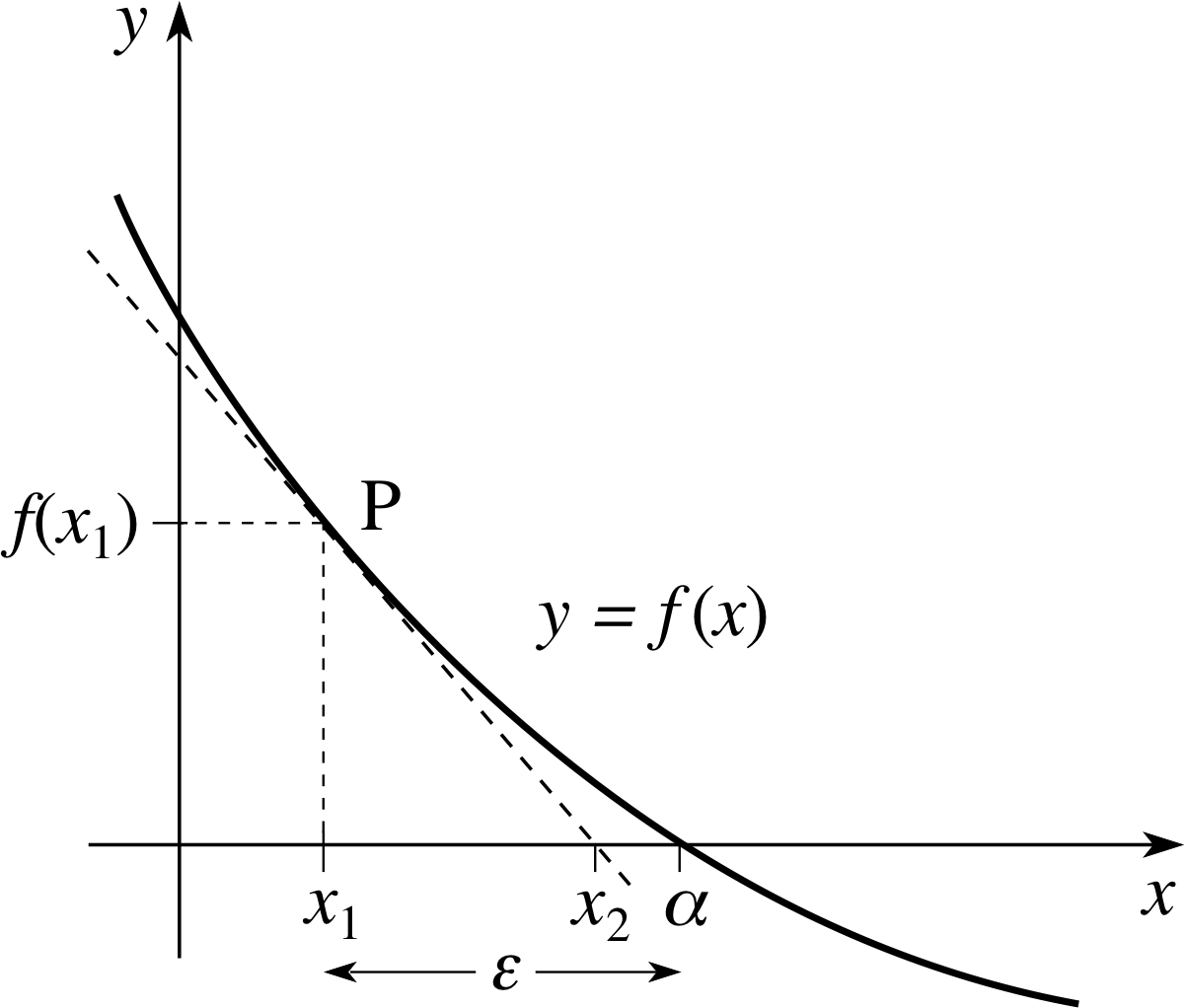
Figure 5 The graph of y = f (x) showing a root at x = α.
First we find the Taylor approximation of degree one about x = x1
y = f (x1) + f ′ (x1)(x − x1)
This is the equation of a line, and it is in fact the equation of the tangent line to the graph of y = f (x) at the point (x1, f (x1)), the dashed line through the point P in Figure 5. This line meets the x–axis at the point (x2, 0), and so
0 = f (x1) + f (x1)(x2 − x1)
which can be rearranged to give the formula
$x_2 = x_1 - \dfrac{f(x_1)}{f'(x_1)}$(43)
Although it appears from Figure 5 that x2 is likely to be a better approximation to the root α than x1, such an argument is unlikely to convince a mathematician and something like the following discussion is required.
Example 3
Show that if x1 is a good approximation for a root of the y equation f (x) = 0, then Equation 43 is (generally) a better approximation to the root. Use this expression to find a better solution of the equation
x2 − 2x − 5 = 0
starting from the approximate solution x ≈ 4.
Solution
Suppose that x1 is a good approximate solution, then the error, ε (see Figure 5) in our approximate solution, is given by ε = α − x1, and ε is small.
Notice that x1 = α − ε, and our intention is to estimate the size of ε, so that we can (partially) correct the error in x1.
Unusually, we regard ε as the independent variable, then consider what happens when we expand an arbitrary function of ε, say F (ε), as a Taylor series (in powers of ε) about ε = 0. From Equation 21,
$f(x) = f(0) + \dfrac{f'(0)}{1!}+ \dfrac{f''(0)}{2!}+ \dfrac{f^{(3)}(0)}{3!}+ \dots + \dfrac{f^{(n)}(0)}{n!}$(Eqn 21)
we have (with ε in place of x)
$F(ε ) = F(0) + F'(0)\dfrac{\varepsilon}{1!} + F''(0)\dfrac{\varepsilon^2}{2}! + \dots$(44)
Now we choose F (ε) to be a particular function of ε, in fact we put i
F (ε) = f (x1 + ε)
so that F (0) = f (x1) and f ′ (0) = f ′ (x1)
and Equation 44 becomes
f (x1 + ε) = f (x1) + εf ′ (x1) + (terms involving ε2 and higher powers of ε)(45)
Remember that x1 + ε = α is a root of the original equation, so that f (x1 + ε) = 0, so that Equation 45 implies that
εf ′ (x1) = −f (x1) − (terms involving ε2 and higher powers of ε) and this gives us an estimate for ε in terms of x1, and the original function, as follows
$\varepsilon = -\dfrac{f(x_1)}{f'(x_1)}$ − (terms involving ε2 and higher powers of ε)(46)
It follows that the true solution
$\alpha = x_1 + \underbrace{~~\varepsilon~~}_{\color{purple}{\large{\substack{\text{this is}\\[1pt]\text{small}}}}} = x_1 - \dfrac{f(x_1)}{f'(x_1)} − \underbrace{(\text{terms involving }\varepsilon^2\text{ and higher powers of }\varepsilon)}_{\color{purple}{\large{\text{this is even smaller}}}}$(Eqn 45)
We know that ε is small and therefore the terms involving ε2 and higher powers of ε must be very much smaller, and so
$x_2 = x_1 - \dfrac{f(x_1)}{f'(x_1)}$
must be even closer to the true solution than our first estimate x1.
The calculation can go wrong if f ′ (x1) is very small, but generally this improved solution can be used as the starting point for the calculation of an even better solution. We therefore have an iterative technique for solving equations, and the iteration can be continued indefinitely and so provide solutions that are as accurate as we please.
In the particular case of f (x) = x2 − 2x − 5 and x1 = 4, we have
f (x1) = 16 − 8 − 5 = 3
andf ′ (x1) = [2x − 2]x=4 = 6
For the first iteration we therefore obtain (from Equation 43)
$x_2 = x_1 - \dfrac{f(x_1)}{f'(x_1)}$(Eqn 43)
$x_2 = 4 - \dfrac{6}{3} = 3.5$
We can now repeat the process and use this value as a starting point for another approximation
$f(x_2) = \dfrac{49}{4} - 7 - 5 = 0.25$
f ′ (x2) = [2x − 2]x=3.5 = 5
and using Equation 43 again
(with x3 in place of x2, and x2 in place of x1) gives us
$x_3 = x_2 - \dfrac{}f(x_2){}f'(x_2) = 3.5 - 0.05 = 3.45$
Continuing in this fashion we could obtain the following approximations to the root
4.0, 3.5, 3.45, 3.449 489 80, 3.449 489 74, ...
and thereafter the first eight decimal places will not change.
If xn is the nth approximation to the root of the equation f (x) = 0, then the next approximation is given by
$x_{n+1} = x_n - \dfrac{f(x_n)}{f'(x_n)}$
This is known as the Newton–Raphson formula.
Since f (x) = 0 is a quadratic equation, the standard formula for such equations gives the exact roots $\alpha = 1 \pm \sqrt{6^\os}$ (The positive root gives good agreement with our result.) i
Question T17
If a function, f (x), is defined by f (x) = x loge(x) − 1 use three iterations of the Newton–Raphson technique, i with the starting value of 2, to find an approximate solution to the equation f (x) = 0.
Answer T17
If x is a good approximation to f (x) = 0, then
$X(x) = x - \dfrac{f(x)}{f'(x)}$
is a better approximation. In this case we have
$X(x) = x - \dfrac{x\log_{\rm e}(x) - 1}{\log_{\rm e}(x) + 1} = \dfrac{x + 1}{\log_{\rm e}(x) + 1}$
The first three iterations give
X (2) ≈ 1.772
X (1.772) ≈ 1.7632
X (1.7632) ≈ 1.763 223
Thermal expansion and anharmonicity
Many materials expand when they are heated, and it is possible to construct a mathematical model which explains why this happens in terms of the behaviour of their molecules. Taylor series are central to this mathematical model, and therefore crucial to an understanding of the mechanism which causes thermal expansion.
Two atoms in close proximity exert forces on each other, rather like the tension or compression in a spring. In the case of atoms the force between them is composed of two components, one of repulsion and one of attraction. The repulsive forces between two atoms, caused by the overlapping of two electron clouds, act over a short range; while the attractive force (the van der Waals force), due to the distortion of the electron cloud of one molecule because of the presence of the other, acts over a rather greater distance.
Just as a stretched spring can store energy, so too can a pair of atoms – energy is required to pull them apart, or to push them together – and this (potential) energy, V say, is a function of the distance r between the atoms. In Figure 6 we show two examples of such functions.
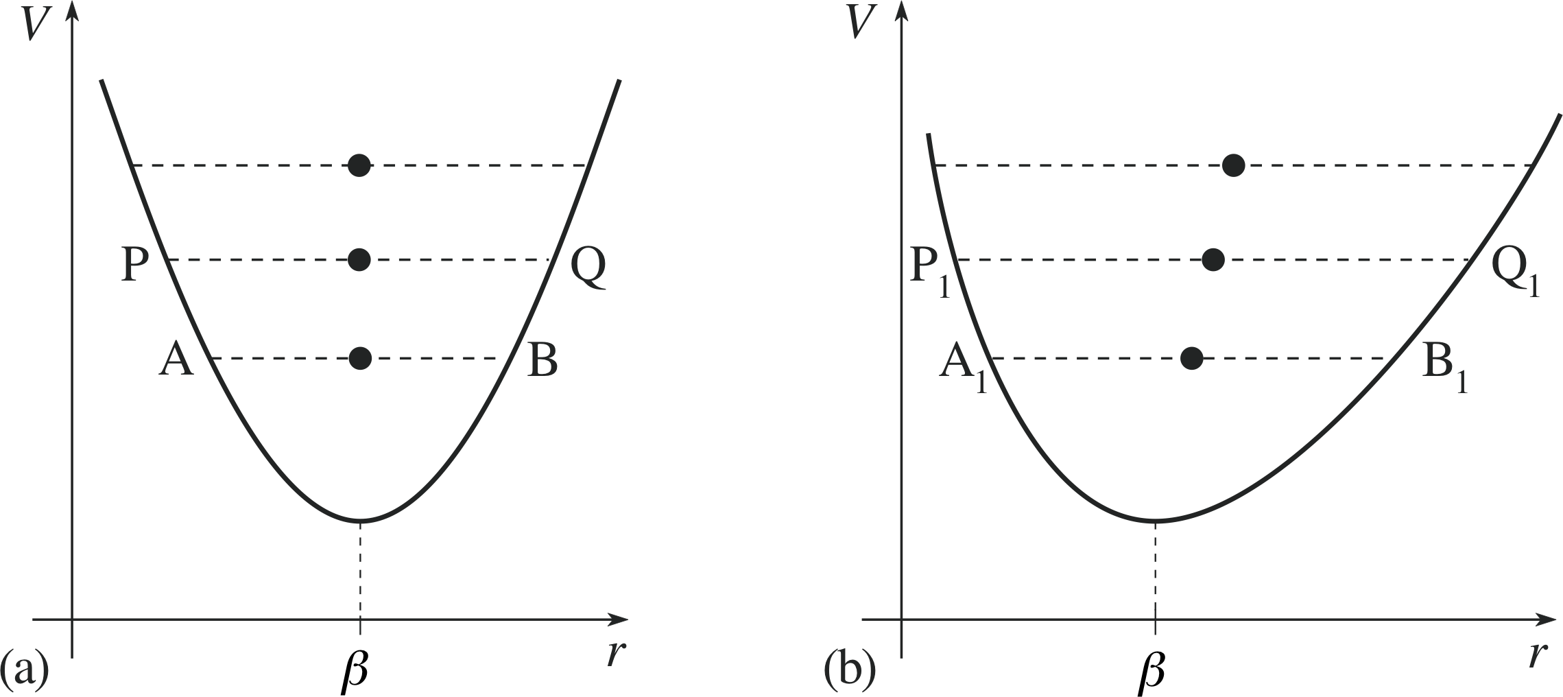
Figure 6 Potential energy V as a function of the distance r between two atoms..
The mid–point of the line AB in Figure 6a represents the mean distance between two atoms at this particular energy level.
Notice that as we increase the energy the mid–point (of the line PQ say) remains directly above the value r = β. Such a case represents a material in which it is just as difficult to push the atoms together as it is to pull them apart, and when they vibrate (which they will do as the temperature rises) they will do so in an harmonic fashion, so that their mean separation remains unchanged. In other words, the material does not expand as the temperature is raised. This corresponds to a graph which is symmetric about the line r = β.
On the other hand, Figure 6b represents the behaviour of a material in which two atoms can be more easily pulled apart than pushed together. In this case the mid–point of the line moves to the right as the energy increases (from the mid–point of A1B1 to the mid–point of P1Q1 say) so that the mean displacement between the atoms increases with temperature, i.e. the material expands. Such systems are said to be anharmonic, and correspond to a graph which is not symmetric about a vertical axis through r = β.
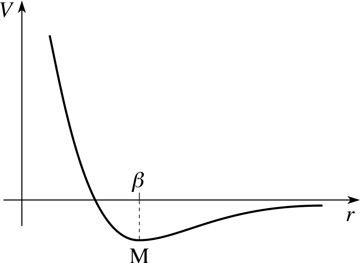
Figure 7 The Lennard–Jones 6–12 function.
The function V (r) may be expanded as a Taylor series about a point β say, so that Equation 34 becomes
$V(r) = V(\beta) + V(\beta)(r - \beta) + V''(\beta)\dfrac{(r - \beta)^2}{2!} V^{(3)}(\beta)\dfrac{(r - \beta)^3}{3!} + \dots$(47)
The potential energy is often modelled by the Lennard–Jones 6–12 function (shown in Figure 7). One form of this function is given below:
$V(r) = \varepsilon\left[\left(\dfrac{a}{r}\right)^{12}-2\left(\dfrac{a}{r}\right)^6\right]$(48) i
where ε and a are constants and r is the distance between the atoms. Such a mathematical model is appropriate for molecular solids, such as argon (and less so for metals).
We will examine the behaviour of this function close to its minimum value at r = β and hence determine how a material modelled by Equation 48 behaves as the energy increases. To do so we will need the first three derivatives of the function V (r) evaluated at the point r = β (bearing in mind that the first derivative must be zero at M because this is a minimum point on the graph).
First we rearrange Equation 48 a little to obtain
$V(r) = 12\varepsilon\left[\dfrac{1}{12}\left(\dfrac{a}{r}\right)^{12}-\dfrac{1}{6}\left(\dfrac{a}{r}\right)^6\right]$
then we use the fact that r = β corresponds to the minimum point on the graph of V (r), so that
$V'(\beta) = -\dfrac{12}{a}\varepsilon\left[\left(\dfrac{a}{r}\right)^{13}-\left(\dfrac{a}{r}\right)^7\right]_{r=\beta} = -\dfrac{12}{a}\varepsilon\left[\left(\dfrac{a}{\beta}\right)^{13}-\left(\dfrac{a}{\beta}\right)^7\right] = 0$
from which it follows immediately that β = a.
Now we differentiate again to find
$V''(\beta) = \dfrac{12}{a^2}\varepsilon\left[13\left(\dfrac{a}{r}\right)^{14}-7\left(\dfrac{a}{r}\right)^8\right]_{r=\beta} = \dfrac{72\varepsilon}{a^2}$ i
and$V^{(3)}(\beta) = -\dfrac{12}{a^2}\varepsilon\left[13\times 14\left(\dfrac{a}{r}\right)^{15}-7\times 8\left(\dfrac{a}{r}\right)^9\right]_{r=\beta} = \dfrac{-1512\varepsilon}{a^3}$
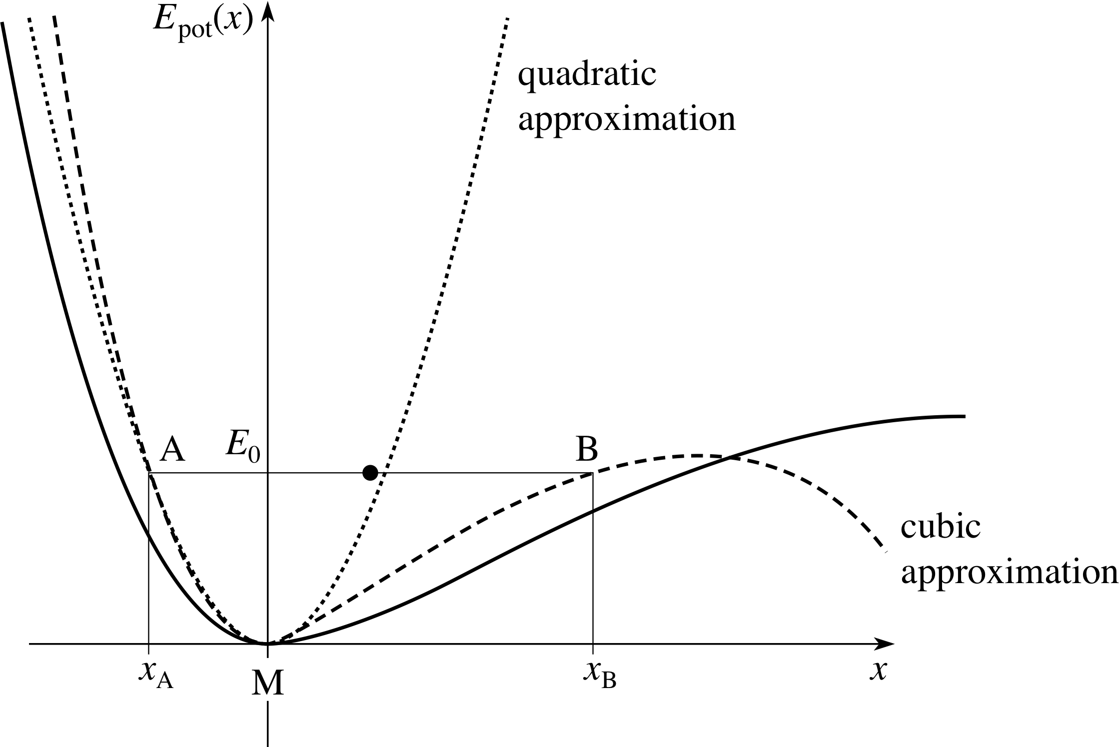
Figure 8 A cubic approximation to Epot(x).
The purpose of these calculations is to simplify Equation 47, and we can simplify it still further if we let x = (r − β) and Epot(x) = V (r) − V (β) to obtain i)
$E_{\rm pot}(x) \approx 36\varepsilon\left(\dfrac{x}{a}\right)^2 - 252\varepsilon\left(\dfrac{x}{a}\right)^3$(49)
and as a further simplification we let P = 36ε and Q = 252ε, so that Equation 49 can be written as
$E_{\rm pot}(x) \approx P\varepsilon\left(\dfrac{x}{a}\right)^2 - Q\varepsilon\left(\dfrac{x}{a}\right)^3$(50)
Effectively this means that we have moved the graph of Figure 7 so that the point M is at the origin, and the right–hand side of Equation 50 is the cubic approximation illustrated in Figure 8.
Now consider a pair of vibrating atoms with fixed total energy E0. At any instant
E0 = Epot(x) + Ekin(x)
where Ekin(x) represents their instantaneous kinetic energy when their separation is r = β + x.
The quantity Ekin(x) must be positive, so the greatest and least possible values of x for the atoms will be given by the roots (i.e. solutions) of the equation E0 = Epot(x), and their approximate values will be given by x = xA and x = xB the solutions of the equation
$E_0 = P\left(\dfrac{x}{a}\right)^2 - Q\left(\dfrac{x}{a}\right)^3$(51)
Once we have found xA and xB, the amount by which the average separation at energy E0 exceeds the minimum energy separation will be given by $\dfrac{x_A + x_B}{2}$.
We can easily obtain a first estimate of xA and xB by ignoring the term involving x3 in Equation 51, so that xA and xB are approximately the roots of the equation $E_0 = P\left(\dfrac{x}{a}\right)^2$.
then $x_{\rm A} = -a\sqrt{E_0}{P}$, $x_{\rm B} = +a\sqrt{E_0}{P}$(52)
and$\dfrac{x_A + x_B}{2} = 0$(53)
This estimate is not sufficiently accurate for our purpose, but the estimates for xA and xB in Equation 52 can be used to obtain an improved estimate as follows. Since xA and xB are roots of Equation 51 we have
$Px_{\rm A}^2 - \dfrac{Q}{a}x_{\rm A}^3 = a^2E_0$(54)
and$Px_{\rm B}^2 - \dfrac{Q}{a}x_{\rm B}^3 = a^2E_0$(55)
Subtracting these equations, and factorizing the result, we obtain
$P(x_{\rm A} - x_{\rm B})(x_{\rm A} + x_{\rm B}) - \dfrac{Q}{a}(x_{\rm A} - x_{\rm B})(x_{\rm A}^2 + x_{\rm A}x_{\rm B} + x_{\rm B}^2) = 0$
and therefore (since xA ≠ xB)
$\dfrac{x_{\rm A} + x_{\rm B}}{2} = \dfrac{Q}{2aP}(x_{\rm A}^2 + x_{\rm A}x_{\rm B} + x_{\rm B}^2)$(56)
Substituting the estimates for xA and xB from Equation 52 into the right–hand side of Equation 56 we obtain
$\dfrac{x_{\rm A} + x_{\rm B}}{2} = \dfrac{Q}{2aP}\left(\dfrac{a^2E_0}{P} - \dfrac{a\sqrt{E_0}}{\sqrt{P}}\dfrac{a\sqrt{E_0}}{\sqrt{P}} + \dfrac{a^2E_0}{P}\right) = \dfrac{aQE_0}{2P^2}$
and after substituting P = 36ε and Q = 252ε we obtain
$\dfrac{x_{\rm A} + x_{\rm B}}{2} \approx \dfrac{7aE_0}{72\varepsilon}$(57)
From Equation 57 it follows that as the energy E0 increases, the mean distance between the atoms also increases, in other words the material expands.
Study comment In this module we have studied Taylor polynomials as approximations to various functions. Such approximations are valuable in certain circumstances, such as obtaining the equation for a simple pendulum near to its equilibrium position. However, it is important that you should realize that in other circumstances a Taylor polynomial may not be the best approximation since it becomes less accurate as we move further away from the point about which we are expanding. You should be aware that there are other polynomial approximations which may be better in some circumstances. However, such polynomials are not considered within FLAP.
4 Closing items
4.1 Module summary
- 1
-
The Subsection 3.1Taylor polynomial of degree n for f (x) near x = 0 is
$p_n(x) = f(0) + \dfrac{f'(0)}{1!}x + \dfrac{f''(0)}{2!}x^2 + \dfrac{f^{(3)}(0)}{3!}x^3 + \cdots + \dfrac{f^{(n)}(0)}{n!}x^n$(Eqn 19)
- 2
-
The Subsection 3.2Taylor series or expansion for f (x) near x = 0 is
$f(x) = f(0) + \dfrac{f'(0)}{1!}+ \dfrac{f''(0)}{2!}+ \dfrac{f^{(3)}(0)}{3!}+ \dots + \dfrac{f^{(n)}(0)}{n!}$(Eqn 21) i
- 3
-
The Subsection 3.3Taylor polynomial of degree n for f (x) near x = a is
$p_n(x) = f(a) + \dfrac{f'(a)}{1!}(x-a) + \dfrac{f''(a)}{2!}(x-a)^2 + \dfrac{f^{(3)}(a)}{3!}(x-a)^3 + \dots + \dfrac{f^{(n)}(a)}{n!}(x-a)^n$(Eqn 31)
- 4
-
The Subsection 3.4Taylor series, or expansion, for f (x) near x = a is
$f(x) = f(a) + \dfrac{f'(a)}{1!}(x-a) + \dfrac{f''(a)}{2!}(x-a)^2 + \dfrac{f^{(3)}(a)}{3!}(x-a)^3 + \dots + \dfrac{f^{(n)}(a)}{n!}(x-a)^n + \dots$
- 5
-
For a convergent series, the error in using a Taylor polynomial is approximately equal to the next (non-zero) term in the corresponding Taylor series.
- 6
-
If xn is the nth approximation to the root of the equation f (x) = 0, then the next approximation is given by
$x_{n+1} = x_n - \dfrac{f(x_n)}{f'(x_n)}$
This is known as the Newton–Raphson formula.
- 7
-
New Taylor series can be found from known series by various methods, including:
- substitution;
- combinations of series;
- differentiation.
4.2 Achievements
Having completed this module, you should be able to:
- A1
-
Define the terms that are emboldened and flagged in the margins of the module.
- A2
-
Use the general form of a Taylor series to find series expansions for given functions about x = 0 or about x = a.
- A3
-
Describe and estimate the approximation involved in replacing a Taylor expansion by the corresponding polynomial.
- A4
-
Derive new Taylor series from known series.
Study comment You may now wish to take the following Exit test for this module which tests these Achievements. If you prefer to study the module further before taking this test then return to the topModule contents to review some of the topics.
4.3 Exit test
Study comment Having completed this module, you should be able to answer the following questions, each of which tests one or more of the Achievements.
Question E1 (A2)
Find the Taylor polynomial of degree 4 for $\sqrt{1 + x}$ near x = 0.
Answer E1
The Taylor polynomial is given by
$\displaystyle p(x) = \sum_{n=0}^4f^n(0)\dfrac{x^n}{n!}$
where f (x) = (1 + x)1/2 and
$\begin{align}f(0) & = \left[(1+x)^{1/2}\right]_{x=0} = 1\\ f'(0) & = \left[\dfrac{1}{2}(1+x)^{-1/2}\right]_{x=0} = \dfrac{1}{2}\\ f''(0) & = \left[\left(\dfrac{1}{2}\right)\left(\dfrac{-1}{2}\right)(1+x)^{-3/2}\right]_{x=0} = \left(\dfrac{1}{2}\right)\left(\dfrac{-1}{2}\right)\\ f^{(3)}(0) & = \left[\left(\dfrac{1}{2}\right)\left(\dfrac{-1}{2}\right)\left(\dfrac{-3}{2}\right)(1+x)^{-5/2}\right]_{x=0} = \left(\dfrac{1}{2}\right)\left(\dfrac{-1}{2}\right)\left(\dfrac{-3}{2}\right)\\ f^{(4)}(0) & = \left[\left(\dfrac{1}{2}\right)\left(\dfrac{-1}{2}\right)\left(\dfrac{-3}{2}\right)\left(\dfrac{-5}{2}\right)(1+x)^{-7/2}\right]_{x=0} = \left(\dfrac{1}{2}\right)\left(\dfrac{-1}{2}\right)\left(\dfrac{-3}{2}\right)\left(\dfrac{-5}{2}\right)\\ \end{align}$
and therefore the Taylor polynomial of degree 4 is
$\begin{align} p(x) & = 1 + \dfrac{x}{2} + \dfrac{1}{2}\left(\dfrac{-1}{2}\right)\dfrac{x^2}{2!} + \dfrac{1}{2}\left(\dfrac{-1}{2}\right)\left(\dfrac{-3}{2}\right)\dfrac{x^3}{3!} + \dfrac{1}{2}\left(\dfrac{-1}{2}\right)\left(\dfrac{-3}{2}\right)\left(\dfrac{-5}{2}\right)\dfrac{x^4}{4!}\\ & = 1 + \dfrac{x}{2} - \dfrac{x^2}{8} + \dfrac{x^3}{16} - \dfrac{5x^4}{128}\end{align}$
(Reread Subsection 3.1 if you had difficulty with this question.)
Question E2 (A2 and A3)
Obtain an approximate value of sin(50°) by taking the first two non–zero terms in the Taylor expansion of sin(x) about x = 45°. Give an estimate of the likely error in your approximation.
Answer E2
The Taylor expansion is
$\displaystyle f(x) = \sum_{n=0}^\infty f^n(0)\dfrac{(x-a)^n}{n!}$
so writing f (x) = sin x (and remembering that x must be measured in radians) we need
$\begin{align} f\left(\dfrac{\pi}{4}\right) & = \sin\left(\dfrac{\pi}{4}\right) = \dfrac{1}{\sqrt{2^\os}}\\ f'\left(\dfrac{\pi}{4}\right) & = \cos\left(\dfrac{\pi}{4}\right) = \dfrac{1}{\sqrt{2^\os}}\\ f''\left(\dfrac{\pi}{4}\right) & = -\sin\left(\dfrac{\pi}{4}\right) = -\dfrac{1}{\sqrt{2^\os}}\end{align}$
The first two terms of the Taylor polynomial are therefore given by
$\sin(x) = \dfrac{1}{\sqrt{2^\os}} + \left(x - \dfrac{\pi}{4}\right)\dfrac{1}{\sqrt{2^\os}}$
Converting from degrees into radians we have
$x - \dfrac{\pi}{4} = (50° - 45°)\times \dfrac{\pi\,{\rm radians}}{180°} = \dfrac{\pi}{36}\,{\rm radians}$
and therefore
$\sin(50°) \approx \dfrac{1}{\sqrt{2^\os}}\left(1+\dfrac{\pi}{36}\right) \approx 0.768\,8135$
with a possible error of
$\dfrac{1}{2!}\left(x-\dfrac{\pi}{4}\right)^2\left(-\dfrac{1}{\sqrt{2^\os}}\right) = -\left(\dfrac{\pi}{36}\right)^2\dfrac{1}{2\sqrt{2^\os}} \approx -0.002\,6925$
These results are consistent with my calculator which gives 0.766 0444 for sin(50°).
(Reread Subsection 3.3 if you had difficulty with this question.)
Question E3 (A2 and A3)
Find the Taylor expansion of loge(x) near x = 1.
Answer E3
Writing
$f(x) = \log_{\rm e} = \displaystyle \sum_{x=0}^\infty f^{(n)}(a)\dfrac{(x-a)^n}{n!}$
we see that we need
$\begin{align} f(1) & = \log_{\rm e}(1) = 0\\ f'(1) & = \left[\dfrac{1}{x}\right]_{x=1} = 1\\ f''(1) & = -\left[\dfrac{1}{x^2}\right]_{x=1} = -1\\ f^{(3)}(1) & = \left[\dfrac{2}{x^3}\right]_{x=1} = 2\\ f^{(4)}(1) & = -\left[\dfrac{2\times 3}{x^4}\right]_{x=1} = -3!\\ \vdots \quad & = \quad\vdots\\ f^{(n)}(1) & = -(-1)^n(n-1)!\end{align}$
Hence the expansion near x = 1 is
$\begin{align} \log_{\rm e}(x) & = (x-1) - \dfrac{(x-1)^2}{2!} + 2\dfrac{(x-1)^3}{3!} - 3!\dfrac{(x-1)^4}{4!} + 4!\dfrac{(x-1)^5}{5!} - \dots -(-1)^n(n-1)!\dfrac{(x-1)^n}{n!}\dots\\ & = (x-1) - \dfrac{(x-1)^2}{2} + \dfrac{(x-1)^3}{3} - \dfrac{(x-1)^4}{4} + \dfrac{(x-1)^5}{5} - \dots -(-1)^n\dfrac{(x-1)^n}{n}\dots\end{align}$
(Reread Subsection 3.4 if you had difficulty with this question.)
Question E4 (A4)
Use the known Taylor expansion for exp(x) about x = 0 to obtain the expansion about x = 1.
Answer E4
Since, for all positive integers n
$\dfrac{d^nx}{dx^n}[\exp(x)] = \exp(x)$
it follows from the general expression for the Taylor expansion about x = a0, with a0 = 1 that
$\exp(x) = \exp(1) + \exp(1)(x - 1) + \exp(1)\dfrac{(x - 1)^2}{2!}$
But, exp(1) = e, so:
$\exp(x) = e\left[1+(x-1) + \dfrac{(x-1)^2}{2!} + \dfrac{(x-1)^3}{3!} + \dots\right]$
In this very special case, we could have obtained the same answer by noting that
$\exp(x) = \displaystyle \sum_{n=0}^\infty\dfrac{x^n}{n!} = 1 + \dfrac{x}{1!} + \dfrac{x^2}{2!} + \dfrac{x^3}{3!} + \dots$
and then using the relation
exp(x) = exp(x − 1) exp(1)
to justify writing
$\exp(x) = e\left[1+(x-1) + \dfrac{(x-1)^2}{2!} + \dfrac{(x-1)^3}{3!} + \dots\right]$
(Reread Subsection 3.5 if you had difficulty with this question.)
Question E5 (A4)
Use the known Taylor expansion for loge(1 − x) to obtain the expansion for $\dfrac{1}{2}\log_{\rm e}\left(\dfrac{1+x}{1-x}\right)$ about x = 0.
Answer E5
We know (from Equation 40) that
$\displaystyle \log_{\rm e}(1-x) = -\sum_{n=0}^\infty\dfrac{x^n}{n} = -x - \dfrac{x^2}{2} - \dfrac{x^3}{3} - \dfrac{x^4}{4} + \dots$
and, replacing x by −x,
$\displaystyle \log_{\rm e}(1+x) = -\sum_{n=0}^\infty\dfrac{(-1)^nx^n}{n} = x - \dfrac{x^2}{2} + \dfrac{x^3}{3} - \dfrac{x^4}{4} + \dots$
and we can use the properties of logarithms to write
$\dfrac{1}{2}\log_{\rm e}\left(\dfrac{1+x}{1-x}\right) = \dfrac{1}{2}\left[\log_{\rm e}(1+x) - \log_{\rm e}(1-x)\right]$
So we have
$\dfrac{1}{2}\log_{\rm e}\left(\dfrac{1+x}{1-x}\right) = x + \dfrac{x^3}{3} + \dfrac{x^5}{5} + \dfrac{x^7}{7} + \dots$
(Reread Subsection 3.5 if you had difficulty with this question.)
Study comment This is the final Exit test question. When you have completed the Exit test go back and try the Subsection 1.2Fast track questions if you have not already done so.
If you have completed both the Fast track questions and the Exit test, then you have finished the module and may leave it here.
Study comment Having seen the Fast track questions you may feel that it would be wiser to follow the normal route through the module and to proceed directly to the following Ready to study? Subsection.
Alternatively, you may still be sufficiently comfortable with the material covered by the module to proceed directly to the Section 4Closing items.