MATH 1.5: Exponential and logarithmic functions |
PPLATO @ | |||||
PPLATO / FLAP (Flexible Learning Approach To Physics) |
||||||
|
1 Opening items
1.1 Module introduction
When the electric charge stored in a capacitor is discharged through a resistor, the rate of flow of charge through the resistor is proportional to the charge remaining on the capacitor. In a population of breeding organisms, the number of offspring produced in a given time, and hence the rate of population growth, is proportional to the size of the population. These processes of electrical discharge and population growth both provide examples of exponential change.
Exponential changes are the subject of Section 2 of this module. Subsection 2.1 introduces some more examples of exponential change and uncovers some of their common characteristics. Subsection 2.2 concerns the rate of change of a quantity and shows how this can be related to the gradient of the tangent_to_a_curvetangent to the graph of that quantity. In particular, by requiring that the rate of change of a quantity should always be equal to the instantaneous value of the quantity itself, we are led to define an exponential function, of the form y (x) = ex, where e is an important mathematical constant, equal to 2.718 (to three decimal places). Subsection 2.3 examines the general mathematical properties of exponential functions, and in Subsection 2.4, exponential functions are used to describe various examples of exponential change, including the decay of radioactive nuclei. Section 2 ends with a more mathematical approach to the definition and evaluation of the number e that involves the concept of a limit.
In Section 3, logarithmic functions (logs) are introduced. We see how logarithms can be expressed in different bases, how the logs of products, quotients and power_mathematicalpowers can be expanded, and how the base of a logarithm can be changed. The antilog function is also introduced, and we look at how logs, antilogs and exponential functions can be handled on a calculator. The module ends with a brief look at how logarithmic functions are used in physics to analyse data that obey an exponential law or a power law.
1.2 Fast track questions
Study comment Can you answer the following Fast track questions? If you answer the questions successfully you need only glance through the module before looking at the Subsection 4.1Module summary and the Subsection 4.2Achievements. If you are sure that you can meet each of these achievements, try the Subsection 4.3Exit test. If you have difficulty with only one or two of the questions you should follow the guidance given in the answers and read the relevant parts of the module. However, if you have difficulty with more than two of the Exit questions you are strongly advised to study the whole module.
Question F1
Plot a graph of y = x2 by evaluating y when x = 0, ±1, ±2, ±3. Estimate the gradient (i.e. slope) at x = 2 by drawing a tangent to the curve.
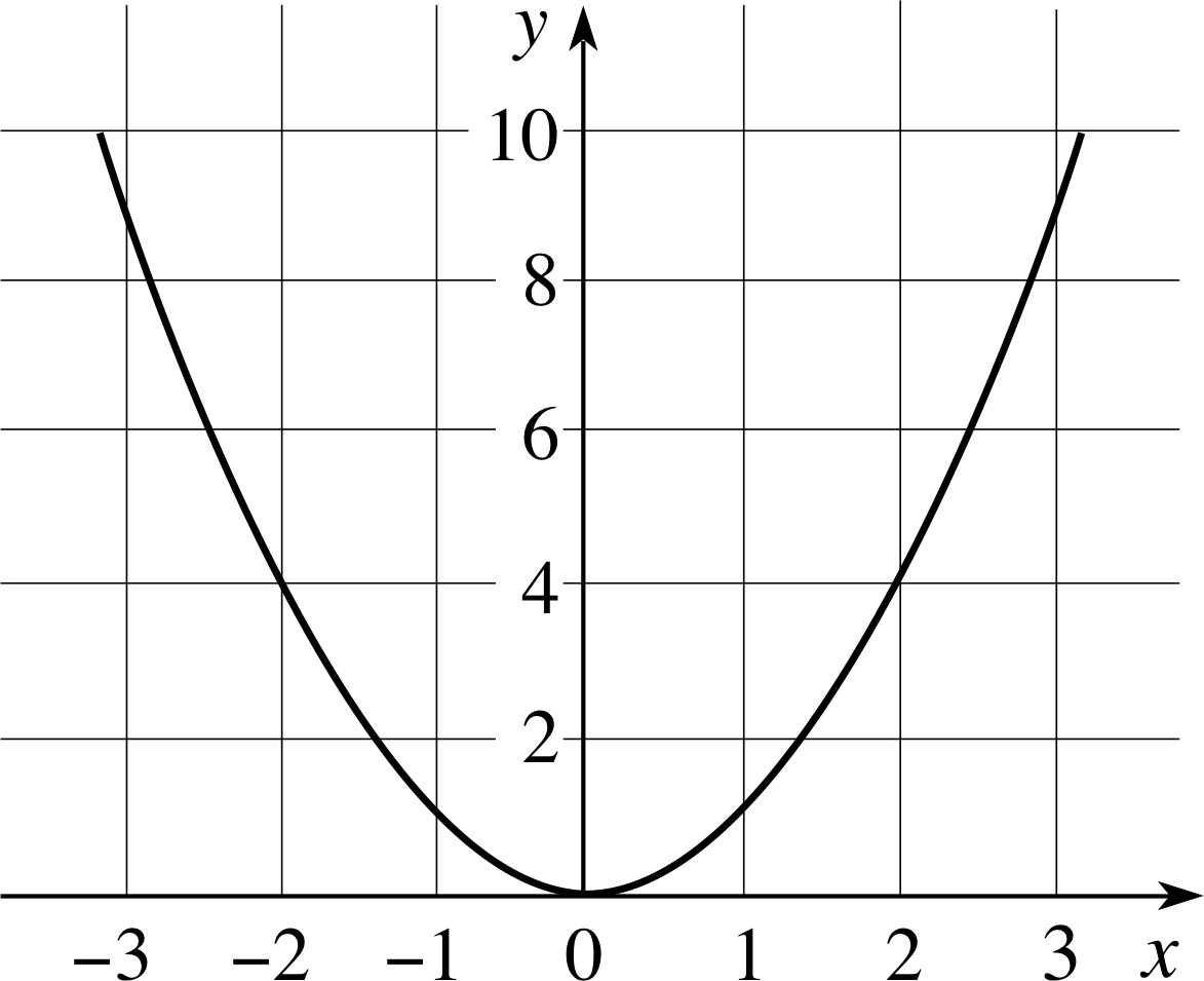
Figure 4 A graph of the equation y = x2.
Answer F1
See Figure 4.
At x = 2 the gradient of the tangent is 4. As this value has been derived from a graph, your value for the gradient may differ slightly from this.
Question F2
Explain what is meant by: $\displaystyle \lim_{x\rightarrow\infty} \frac 1 x$
Answer F2
$\displaystyle \lim_{x\rightarrow\infty}$ is an instruction to evaluate the expression that follows as x tends to infinity.
In this case 1/x tends to 0 as x tends to infinity.
Question F3
State the usual symbol for the following expression, and give its value to three decimal places: $\displaystyle \lim_{m\rightarrow\infty} (1+1/m)^m$
Answer F3
e = 2.718 ... (to three decimal places).
Question F4
What is the gradient of the graph of y = exp(kx) at x = 0?
Answer F4
The gradient is k.
Question F5
Where possible, simplify the following expressions:
(a) loge [(ex) y] (b) loge (ex + e2y) (c) exp[loge (x) + 2 loge (y)] (d) exp[2 loge (x)] (e) a loga (x)
Answer F5
(a) loge [(ex) y] = loge (exy) = xy
(b) This equation cannot be simplified
(c) exp[(loge (x) + 2 loge (y)] = exp[(loge (x)] × exp[(loge (y2)] = xy2
(d) exp[2 loge (x)] = exp[loge (x2)] = x2
(e) aloge (x) = x
Question F6
If P = k f−a, what are the gradient, and the intercept on the vertical axis, of the graph of log10 (P) (plotted vertically) against log10 (f)?
Answer F6
log10 (P) = −a log10 (f) + log10 (k), thus, a graph of log10 (P) against log10 (f) is a straight line of gradient −a and intercept log10 (k).
Study comment Having seen the Fast track questions you may feel that it would be wiser to follow the normal route through the module and to proceed directly to the following Ready to study? Subsection.
Alternatively, you may still be sufficiently comfortable with the material covered by the module to proceed directly to the Section 4Closing items.
1.3 Ready to study?
Study comment In order to study this module you will need to understand the following terms: constant of proportionality, decimal places, dependent variable, dimensions, function, independent variable, index, inverse function, power_mathematicalpower, proportional, reciprocal and root. You will need to be able to use SI units, perform simple algebraic and numerical calculations (including using a calculator), plot the graphs of simple functions, and determine the gradient of a straight line that may be specified graphically or algebraically. If you are uncertain about any of these terms you can review them by referring to the Glossary, which will indicate where in FLAP they are developed. The following questions will allow you to establish whether or not you need to review some of the topics before embarking on this module.
Question R1
Write the following expressions in their simplest form:
(a) $ \underbrace{a \times a \times a \times \dots \times a}_{\color{purple}{\large{m \rm\ factors}}}$ (b) 50
Answer R1
(a) a m (b) 50 = 1
Question R2
If a is any positive number, what is the value of x in the equation: (a4)5 × (a2)3 = a x ?
Answer R2
The expression reduces to a20 × a6 = a26. So x = 26.
Question R3
Write the following expressions in their simplest form:
(a) 16−1/4 (b) 163/4 (c) 45/2 (d) 27−2/3 (e) 1/(3−2)
Answer R3
(a) 16−1/4 = (24)−1/4 = 2−1 = 1/2 (b) 163/4 = (24)3/4 = 23 = 8 (c) 45/2 = (22)5/2 = 25 = 32
(d) 27−2/3 = (32)−2/3 = 3−2 = 1/9 (e) 1/(3−2) = 32 = 9
(If you had difficulty with Questions R1 to R3, refer to power_mathematicalpowers in the Glossary.)
Question R4
If y is a function of x, given by: y = F (x), what is meant by saying that G (x) is its inverse function?
If F (x) = x3, what is G (x)?
Answer R4
The inverse function G (x) ‘undoes’ the effect of F (x), so G [F (x)] = x, for any value of x in the domain of F (x). If F (x) = x3, then G (x) = x1/3.
Question R5
Plot a graph of y = x2 by evaluating the right–hand side of the equation at the points x = 0, ±1, ±2, ±3. Use your graph to find solution_mathematicalsolutions of the equation x2 = 2.72
Figure 4 See Answer R5.
Answer R5
The graph of y = x2 is given in Figure 4. The approximate solution_mathematicalsolutions are x = 1.65 and x = −1.65.
Question R6
Which of the following expressions will give a straight line when y is plotted against x? For those that will give a straight line, state the value of its gradient. (All symbols except y and x represent non–zero constants.)
(a) y = mx + c (b) y = ax2 + b (c) y + x = k (d) y/x = p (e) y/x = qx + r
Answer R6
The expressions in (a), (c), and (d) will give straight–line graphs. The gradients of these graphs are: (a) m, (c) −1, and (d) p.
Question R7
What is the gradient of the straight line joining the points with Cartesian coordinates (1, 5) and (3, 13)?
Answer R7
The ‘rise’ is 8 (= 13 − 5) and the ‘run’ is 2 (= 3 − 1) so the gradient (= rise/run) is 4.
(If you had difficulty with Questions R4 to R7, refer to function, gradient or graph in the Glossary.)
2 Exponential functions
2.1 Exponential growth and decay
In physics, and elsewhere, we are often concerned with how a quantity changes with time. The following examples all have an important feature in common. As you read, think what that feature might be.
Example 1
Suppose that you were to invest £100 with a bank at an interest rate of 5% per year. At the end of the first year your money would have earned £5 in interest, and your total investment would be worth £105. To find the value of your investment after a further year, you would add 5% of £105 (i.e. £5.25) to obtain a total of £110.25 – and so on. Year after year, your total investment would increase, and so would the annual interest, since it would grow in proportion to your total investment. Thus, on an annual basis, the rate of growth of your investment (i.e. the interest gained per year) is proportional to your total investment.
Example 2
When the electric charge Q stored in a capacitor is discharged through a resistor, the rate at which charge leaves the capacitor and flows through the resistor is described by the electric current I through the resistor. The size of this current is determined by the resistance R and the voltage V across the resistor: I = V/R. i However, V itself depends on the capacitance C and the charge Q remaining in the capacitor: V = Q/C. It follows that I = Q/(RC). So, at any moment, the rate at which charge is lost from the capacitor, I, is proportional to the charge, Q, remaining in the capacitor.
Example 3
The ‘activity’ of a radioactive sample is a measure of the number of atomic nuclei in that sample that disintegrate per second. i Since each disintegration effectively removes one unstable nucleus from the sample it is also a measure of the rate at which unstable nuclei are lost from the sample. Now any individual nucleus is equally likely to decay in each second of its lifetime, so the number of disintegrations occurring in a sample in one second will be proportional to the number of unstable nuclei in that sample. Thus, at any time, the rate of decrease in the number of the unstable nuclei in a sample is proportional to the number of unstable nuclei that remain.
✦ What do the above examples have in common?
✧ Each describes a situation where the rate of change of some quantity at a given time is proportional to the value of that quantity at that time.
All the changes discussed above are examples of exponential changes. Such change may cause a quantity to increase (e.g. to grow) or to decrease (e.g. to decay), and may be characterized in the following way:
In an exponential change the rate of change of some quantity, y, at any time t, is directly proportional to the value of y itself at that time:
rate of change of y (t) ∝ y (t) i
i.e.rate of change of y (t) = ky (t)(1)
where k is a constant of proportionality.
If k is positive, y increases with time – this kind of change is called exponential growth.
If k is negative, y decreases with time – this kind of change is called exponential decay.
In our first example, the constant k was simply the interest rate, so, k = 0.05 year−1 (i.e. 5% per year). In the third example, the case of radioactive decay, the rate of change in the number of unstable nuclei was negative since the change reduced the number of such nuclei in the sample. i In such cases the constant of proportionality is usually written as −λ, where λ is a positive quantity called the decay constant – for example, a certain isotope of polonium has a decay constant of λ = 0.0133 s−1. Notice that the units of the decay constant reflect the units of the time interval used to define the rate.
Question T1
How many nuclear disintegrations per second would you expect from a sample containing 6.0 × 10¹⁸ polonium nuclei (λ = 0.0133 s−1)?
Answer T1
Number of disintegrations per second is given by λ × number of polonium nuclei = 0.0133 s−1 × 6.0 × 102 = 8.0 × 10² s−2.
(In fact, this only represents the average number of decays per second, since nuclear decay is a statistical process in which it is not possible to predict the exact number expected in any particular second.)
Question T2
In the second example above, what is the constant of proportionality relating the rate of discharge, I, of a capacitor to the charge Q remaining on the capacitor?
Answer T2
k = −1/(RC). The rate of discharge is equal to the current, I = Q/(RC), and Q is decreasing with time so k must be negative.
There are many examples of exponential change in physics, some of which you will meet during this module. All exponential changes have an underlying mathematical similarity, and later in this section we will develop some powerful mathematical ideas and techniques relating to such changes. First, though, we need to have a more careful look at the idea of a rate of change.
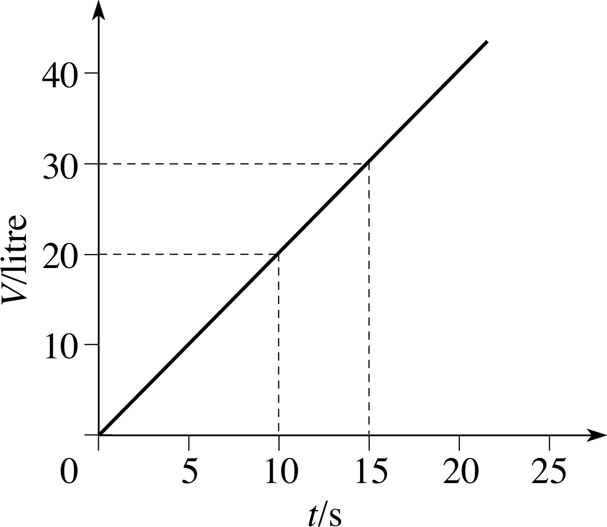
Figure 1 The volume of water in a bath that fills at a constant rate.
2.2 Gradients and rates of change
Figure 1 illustrates how the volume, V, of water increases with time when a bath is filled. You can see from the graph that the water from the tap is running at a constant rate, because the volume of water increases by equal amounts in equal time intervals, i.e. by 2 litres in each second – the rate of change of volume is therefore 2 litres s−1. i
✦ What is the gradient of the graph in Figure 1? What is the relationship between the gradient and the rate of change of volume?
✧ The gradient is 2 litres s−1. The gradient of the graph is equal to the rate of change of volume.
✦ What would the graph look like if the bath were emptying at a constant rate of 5 litres s−1?
✧ The graph would still be a straight line, but sloping in the opposite direction, and steeper. Its gradient would therefore be negative, −5 litres s−1.
We can generalize the above discussion to any constant rate of change:
For any quantity y that changes at a constant rate, the graph of y against time t is a straight line with a gradient equal to the rate of change of y.
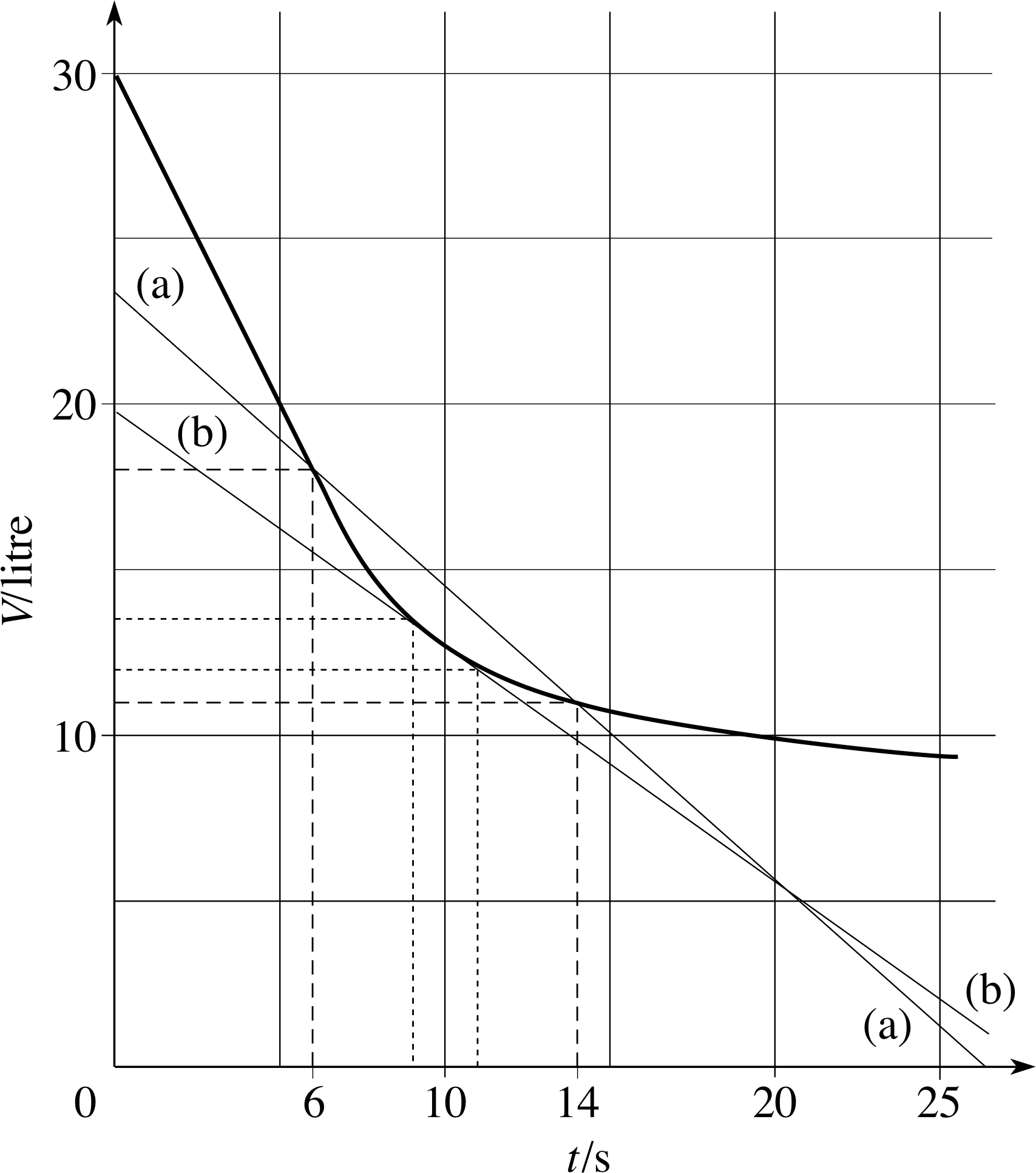
Figure 2 The volume of water in a bath emptying at a decreasing rate. The lines (a) and (b) are used to estimate the flow rate at t = 10 s.
In practice, a bath does not continue to empty, unaided, at a constant rate. As the water level falls, the water pressure also falls, and so the rate at which water flows out of the bath decreases. Figure 2 shows how the volume of water in an emptying bath might change with time. The graph drops steeply at first, corresponding to a rapid flow, and gradually becomes shallower as the flow rate diminishes. i
As before, we can relate the rate of change of volume to the steepness of the graph, even though the steepness is changing from moment to moment, but how do we do this? What feature of a curved graph such as in Figure 2 will let us work out the rate of change of the plotted quantity at any time? We could get a rough value for the rate of change of volume at, say, t = 10 s by finding the change in the volume of water in the bath between t = 6 s and t = 14 s (about −7 litres) and then dividing that volume by the time interval of 8 s (14 s − 6 s) to get a rate of change of volume of about −0.9 litres s−1. This is equivalent to finding the gradient of the straight line joining the points onthegraphatt = 6 s and t = 14 s. Or we could choose a shorter time interval, say 2 s, between t = 9 s and t = 11 s. You can see from the lines (a) and (b) drawn on Figure 2 that a different choice of time interval gives a straight line with a different gradient, and hence a different rate of change of volume. The difference arises because the flow rate is changing during the time intervals and what we have calculated is an average rate of change of volume over each of the specified periods. But how can we improve on this to find the rate of change at a particular time?
If we make the time interval very small indeed, we can hope that the flow rate hardly changes at all during that interval. Instead of a line joining two well–separated points on a curve, the situation is more like that shown in Figure 3; there will be single straight line that just touches the curve at t = 10 s, the steepness of which matches exactly that of the curve at that point. Such a line is called a tangent_to_a_curvetangent to the curve. Using this idea we can define the gradient of the curve, at any particular point, to be the gradient of the tangent to the curve at that particular point. This gradient tells us the instantaneous rate of change at our chosen value of t, rather than the average rate of change over an interval.
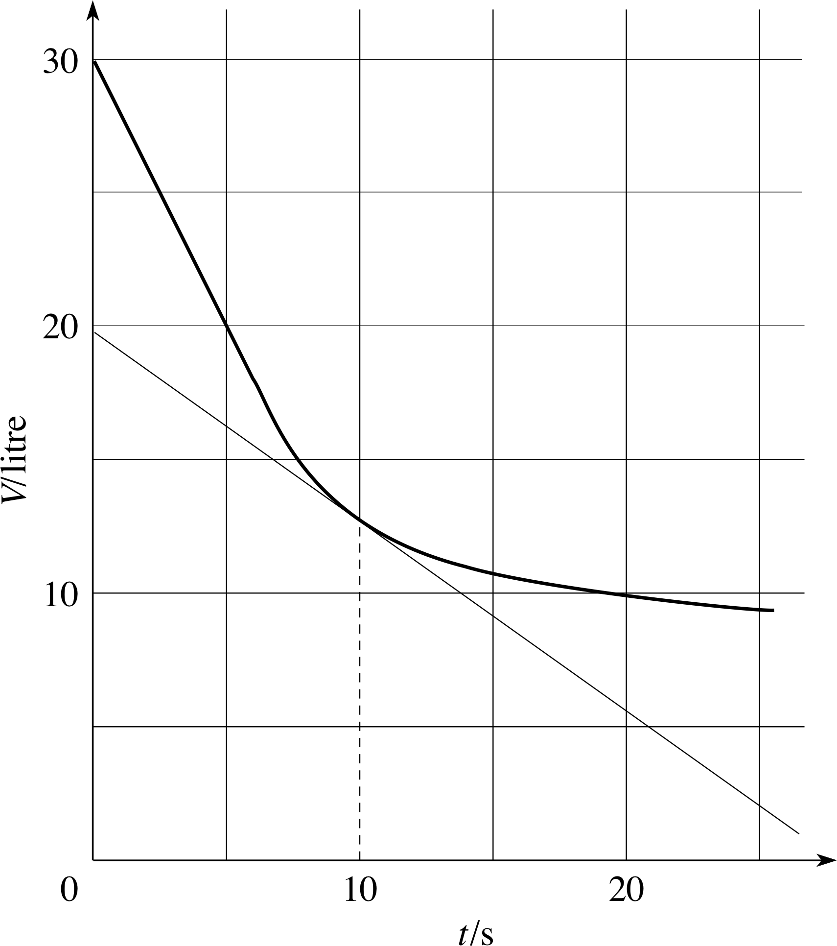
Figure 3 Finding the gradient at a point on a curve by drawing a tangent.
So, if we have a change in volume ∆V in a time interval ∆t, the quantity ∆V/∆t will be equal to the average rate of change of volume during the interval ∆t. i But if we make ∆t and ∆V smaller and smaller we can reasonably expect that ∆V/∆t will provide an increasingly good estimate of the gradient of the tangent. Indeed, if ∆t and ∆V are small enough i, we can expect ∆V/∆t to represent the (instantaneous) rate of change of V.
In the remainder of this module we will use the notation ∆V/∆t to represent the instantaneous rate of change of V with respect to t. i In other words, no matter what value of t we are discussing, we will always assume that we can find suitable values ∆t and ∆V to ensure that ∆V/∆t provides an accurate value for the gradient of the tangent at that value of t. From a strictly mathematical point of view this is not always justified, nor is it a particularly good use of notation, but we shall use it none the less.
When trying to find an instantaneous rate of change from a graph you will probably have to make your best guess at an appropriate tangent, evaluate its gradient as accurately as possible, and accept that by working graphically you are limited to making estimates of rates of change. (Fortunately, there are algebraic techniques that enable us to work out rates of change accurately, but these too belong to the subject of differentiation and will not be developed in this module.)
Question T3
Find the gradient of the tangent at t = 10 s shown in Figure 3. Draw a tangent to the curve at t = 5 s and hence estimate ∆V/∆t when t = 5 s.
Answer T3
For the tangent at t = 10 s, the ‘rise’ ≈ −20 and ‘run’ ≈ 28, so the gradient ≈ −20/28 ≈ −0.71, so the flow rate ∆V/∆t ≈ −0.71 litre s−1. The line passing through t = 0 s, V = 30 litre, and t = 15 s, V = 0 litre, is an approximate tangent to the curve at t = 5 s, so ∆V/∆t ≈ −2 litre s−2. (The exact value you find will depend on how you draw the tangent. )
The above discussion can be generalized to the rate of change of any quantity:
The rate of change of any quantity y, at a particular time, can be represented by the quotient ∆y/∆t, provided the changes ∆y and ∆t are sufficiently small. The value of such a rate of change is given by the gradient of the tangent to the graph of y against t at the time in question.
Furthermore, the idea of a gradient of a curved graph is not confined to graphs showing variation with time.
Figure 4 A graph of the equation y = x2.
✦ Figure 4 is a graph of the equation y = x2. By drawing tangents to the curve, estimate ∆y/∆x when x = 0, x = 2 and x = −1.
✧ At x = 0, you can see from the symmetry of the curve that the gradient is 0. The gradients of the other two tangents are 4 and −2, respectively, though your own results might be slightly different from these values since they will depend on how accurately you draw the tangents.
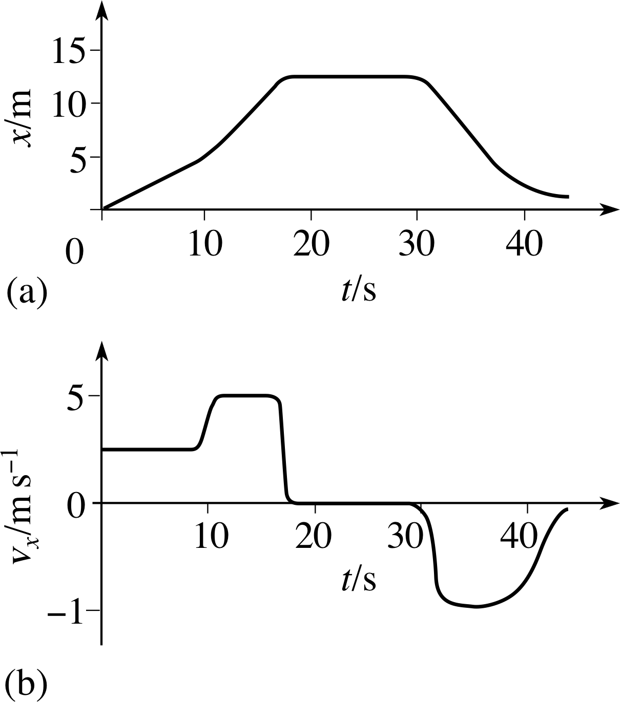
Figure 5 Graphs of (a) the position coordinate and (b) the instantaneous velocity of an object moving along a straight line.
Before we end this subsection, we will have a brief look at some more rates of change and their physical interpretations. One example is shown in Figure 5a, where the graph shows how the position coordinate, x, of an object moving along a straight line, changes with time. This is called linear motion. i Where the graph is steep, the position changes rapidly with time – i.e. the object moves quickly – and shallower parts of the graph correspond to the object moving more slowly. A negative gradient corresponds to the object moving in the reverse direction.
We can therefore say that, at any particular time, the gradient of this position–time graph is equal to the instantaneous velocity vx of the object. Figure 5b shows how the velocity, vx, of the object represented in Figure 5a changes with time.
✦ Suggest a physical interpretation of the gradient of Figure 5b.
✧ The gradient is ∆vx /∆t, the rate of change of velocity, which is equal to the acceleration.
Using the notation introduced above, we can rewrite the condition for exponential change (Equation 1) as:
In an exponential change, at any time ∆y/∆t = ky(2)
Figure 6 shows an example of a quantity that is changing exponentially: N, the number of unstable nuclei in a radioactive sample, decays exponentially with time t. The gradient of the curve at any particular time is equal to the number of disintegrations per second occurring at that time. By drawing tangents to the graph at various times and measuring their gradients it is easy to see that the gradient is indeed proportional to N, as required. When N = 10 × 1010, 6 × 10¹⁰ and 2 × 10¹⁰, the measured gradients are −5 × 10⁴ s−1, −3 × 10⁴ s−1 and −1 × 10⁴ s−1.
Figure 7 shows how the charge Q (measured in coulombs) stored in a capacitor changes with time. By measuring the gradients of tangents at various times, we can find the rate of flow of charge, i.e. the current, at these particular times.
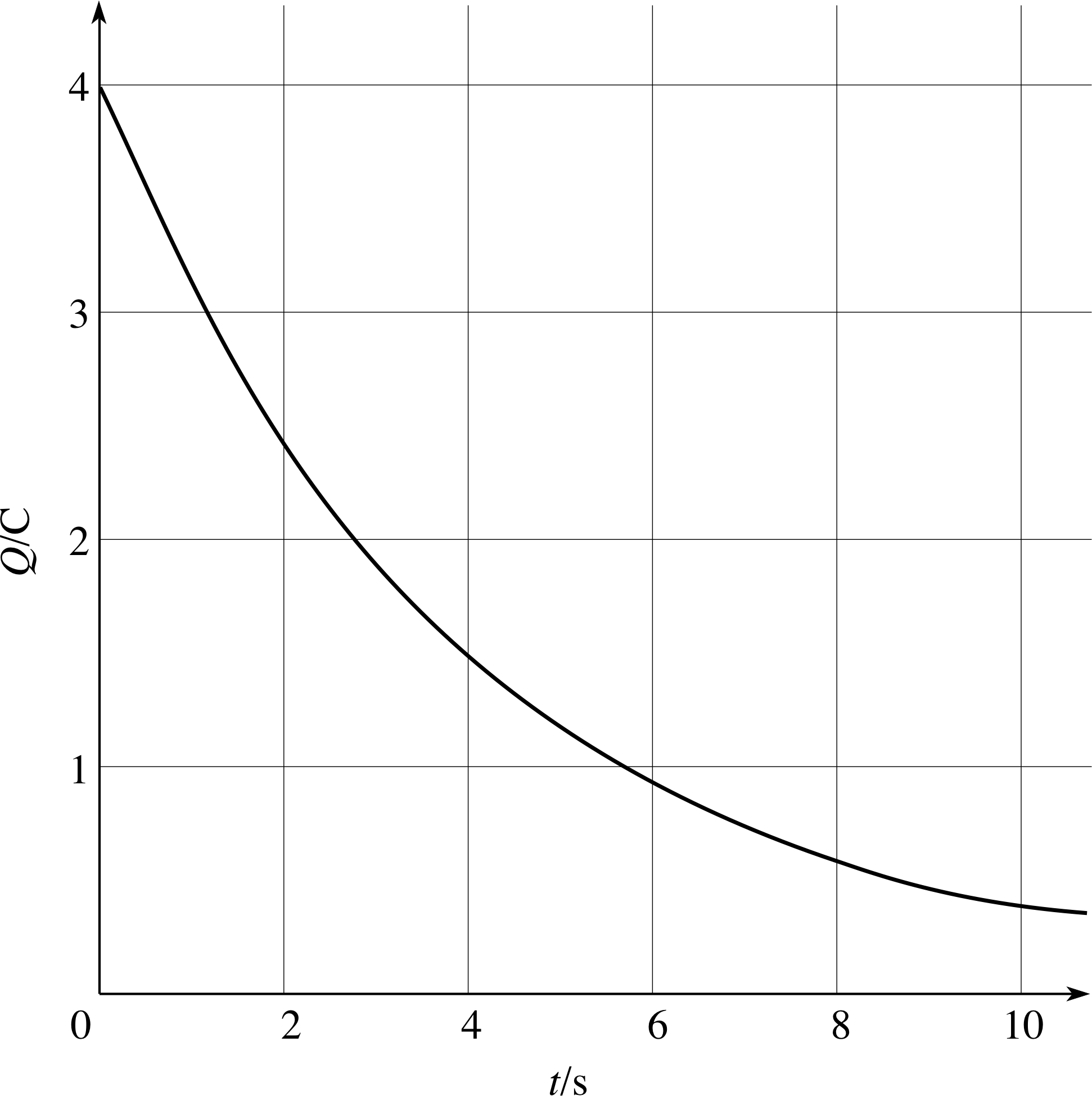
Figure 7 The charge remaining on a discharging capacitor. Another example of exponential decay.
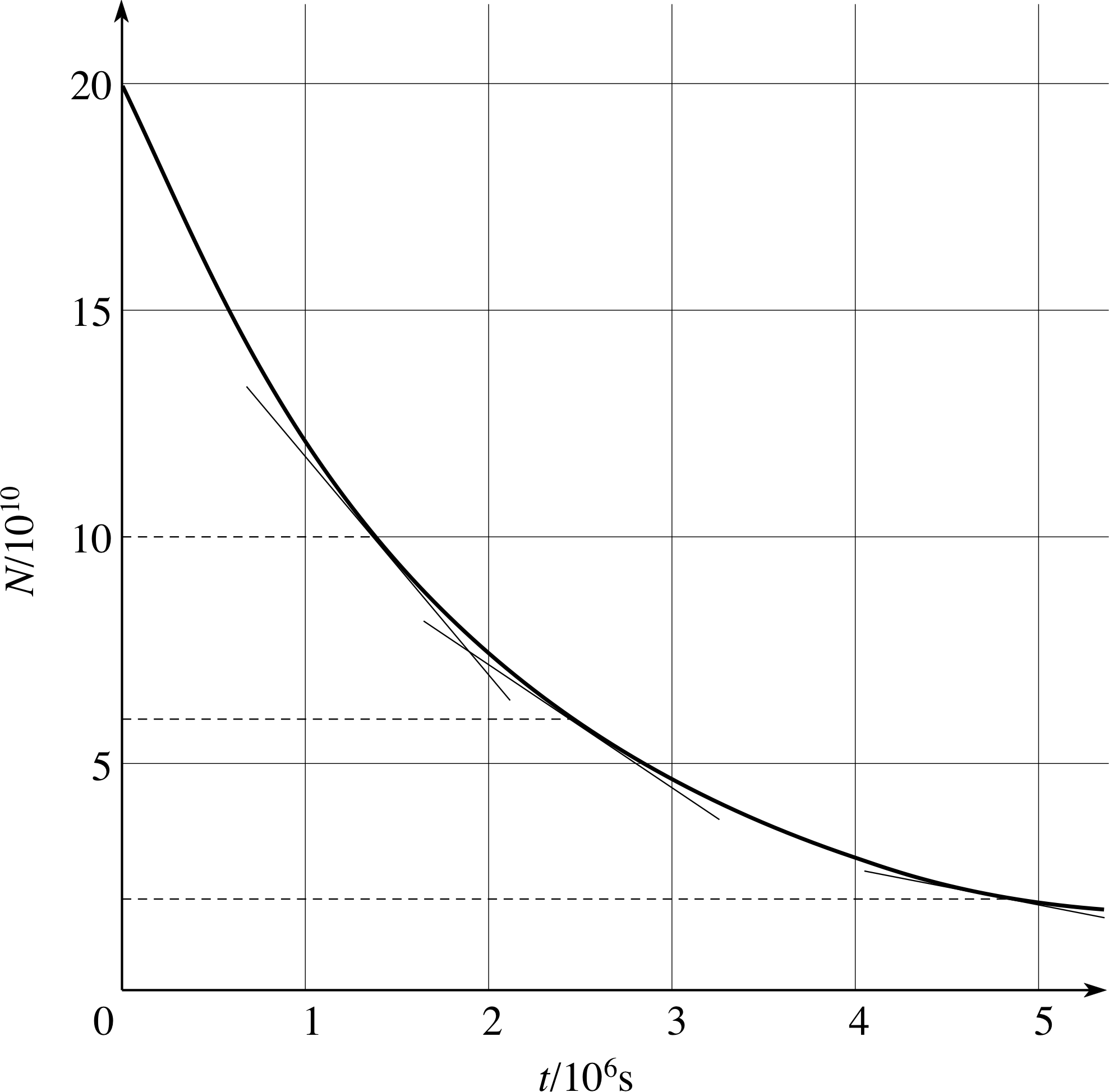
Figure 6 The number of unstable nuclei in a radioactive sample plotted against time, with tangents drawn at N = 10 × 1010, 6 × 10¹⁰ and 2 × 10¹⁰. This is an example of exponential decay.
Question T4
By drawing tangents to the curve, estimate the currents when Q = 2 C, 1 C and 0.5 C, and hence verify that Figure 7 shows exponential decay.
Answer T4
The accurate values for the currents determined for the tangents are 0.5 A, 0.25 A and 0.125 A, i.e. ∆Q/∆t ≈ 0.25 s−1 × Q. (Your values should approximate these.)
Therefore the decay is exponential.
(Of course, rather imprecise measurements made at a few points on a graph do not really verify that the graph is exponential, but at least they haven’t shown any evidence to the contrary, or rather, they shouldn’t have done so!)
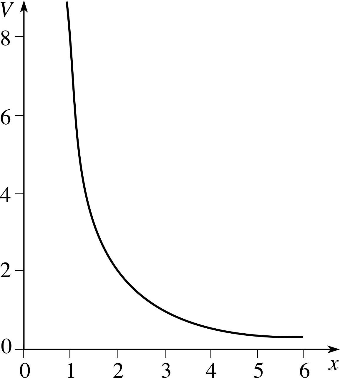
Figure 8 See Question T5.
Question T5
Figure 8 shows the graph of V = 8/x2. Explain how you would show that this curve does not describe exponential decay.
Answer T5
One way would be to show that the gradient is not proportional to the value of V. For instance, you could measure the gradient at x = 1 (where V = 8) and at x = 2 (where V = 2) and show that the gradients at those two points, −16 and −2, respectively, are not in the ratio 8 : 2.
2.3 Exponential functions and the number e
In this subsection, you will learn how to write functions representing the values of quantities that change exponentially. We will begin with exponential growth, since we can then deal entirely with positive quantities. i We will look for a function y (x) such that, at any value of x, the rate of change of y is equal to the value of y itself, i.e. we will look for a function y (x) such that ∆y/∆x = x. For the sake of simplicity we will treat x as a purely numerical variable.
In Subsection 2.1, we saw that when there is a constant annual interest rate the value of an investment grows exponentially. With an interest rate of 5% per year, the value after one year is found by multiplying the initial sum by 1.05 and, after two years, by multiplying again by 1.05, i.e. in two years the value of the initial investment increases by a factor of (1.05)2. If the investment is left for n years at the same interest rate, its initial value will be multiplied by a factor of (1.05) n.
The above example suggests that we should look at functions of the form y (x) = y0a x, where y0 is the initial value of y and a is some (positive) constant number. It may therefore be helpful at this point to have a brief reminder of the properties of such functions.
For any numbers a, x and y:
a xa y = a x+y(3)
(a x) y = a xy(4)
$\displaystyle a^{-x} = \frac{1}{a^x}$(5)
a x/y = (a1/y) x(6) i
Also, recall that a0 = 1 and that by a1/k (for k a positive integer) we mean the kth root of a, i.e. a solution of the equation x k = a.
| x | 2x |
|---|---|
| −3.5 | 0.09 |
| −3.0 | 0.13 |
| −2.5 | 0.18 |
| −2.0 | 0.25 |
| −1.5 | 0.35 |
| −1.0 | 0.50 |
| −0.5 | 0.71 |
| 0 | 1.00 |
| 0.5 | 1.41 |
| 1.0 | 2.00 |
| 1.5 | 2.83 |
| 2.0 | 4.00 |
| 2.5 | 5.66 |
| 3.0 | 8.00 |
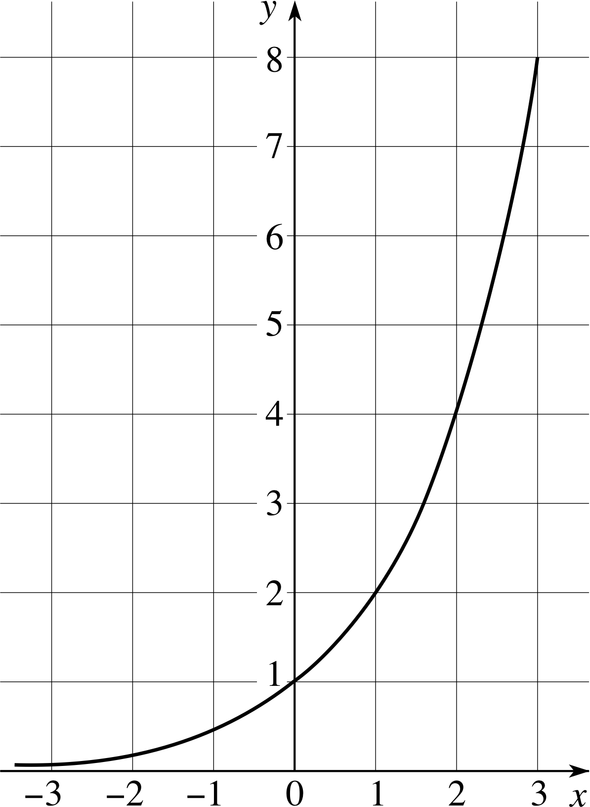
Figure 9 The graph of y (x) = 2x.
Now let us look at a particular function: y (x) = 2x. Figure 9 shows the graph of this function, and Table 1 shows its value for various values of x.
✦ Find the gradients of tangents to the graph of y = 2x at x = −1, 0, 1 and 2. Is this function growing exponentially?
✧ At the given values of x the gradients are approximately 0.7, 1.4 and 2.8, respectively. From Table 1 the corresponding values of y are 1.0, 2.0 and 4.0. So, the gradient apparently increases in proportion to the value of the function. This indicates that y (x) = 2x increases exponentially with increasing x.
In fact the gradient is consistent with ∆y/∆x ≈ 0.7y, not with ∆y/∆x = y. If you were to plot the graph of y (x) = 3x you would find that it too grows exponentially, with a gradient approximately equal to 1.1 × 3x. This suggests that there may be some number a between 2 and 3 such that if y (x) = a x, then the gradient would be exactly equal to the value of y.
It turns out that there is indeed such a number. To three decimal places its value is 2.718, but like π and 2, it is an irrational number i that cannot be accurately represented by any decimal with a finite number of decimal places. For this reason it is conventional to represent its accurate value by the letter e and simply substitute an appropriate numerical value whenever necessary. e is one of the most important numbers in physics and in mathematics. i
e = 2.718 281 828 459 05 ... (to 14 decimal places)
Ify (x) = ex(7) i
then the rate of change ∆y/∆x = y (x)
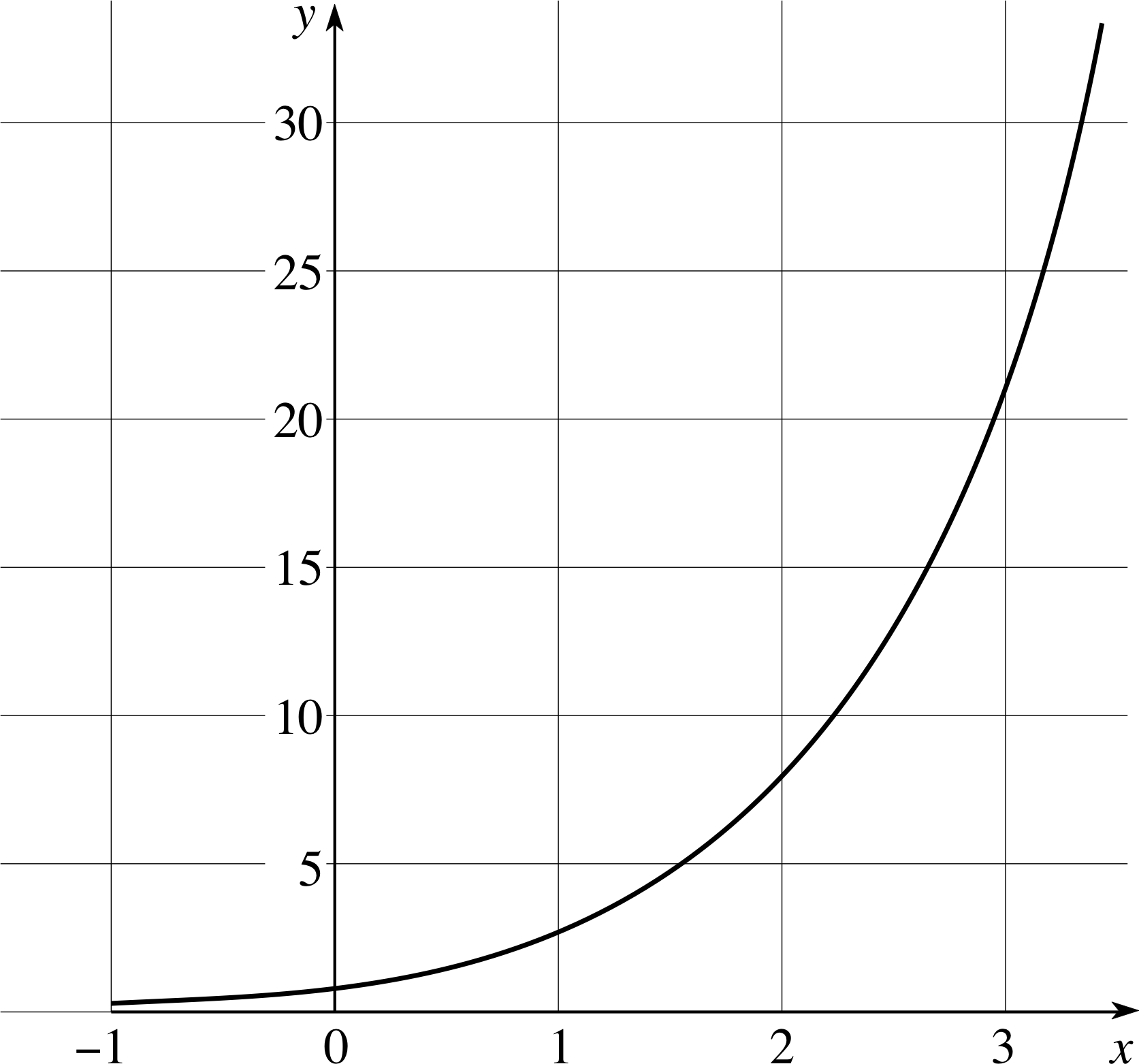
Figure 10 The graph of the function y (x) = ex.
✦ Figure 10 is a graph of y (x) = ex. Draw tangents at a few different points on the graph and measure their gradients. Confirm that at each point you examine the gradient is equal to the value of y.
✧ You should have found that each gradient is close to the value of y (x), thus confirming that the function satisfies ∆y/∆x = y.
The function ex is known as the exponential function, and to emphasize that it is a function of x it is often written as exp(x). i So far, we have used it to describe how something varies with x, where x can be any variable without dimensions (since powers are always dimensionless numbers).
To evaluate exponential functions on a calculator, use the ex key (possibly labelled exp(x)) or its equivalent. i If your calculator does not have such a key, you may be able to calculate ex by using the y x key with y = 2.718, but you are probably best advised to buy a new calculator. i
Question T6
Evaluate e2, e3, e1.43, e−1 and e0.
Answer T6
e2 = 7.389, e3 = 20.09, e1.43 = 4.179, e−1 = 0.3679 (all to four significant figures).
e0 = 1 (a0 = 1 for all values of a).
2.4 Exponential functions and exponential change
So far, you have seen that the function y (x) = exp(x) describes exponential changes in which the rate of change is equal to y (x) at any given value of x. In this subsection, we will see how exponential functions can be used to describe exponential changes that correspond to any value of k in ∆y/∆x = ky.
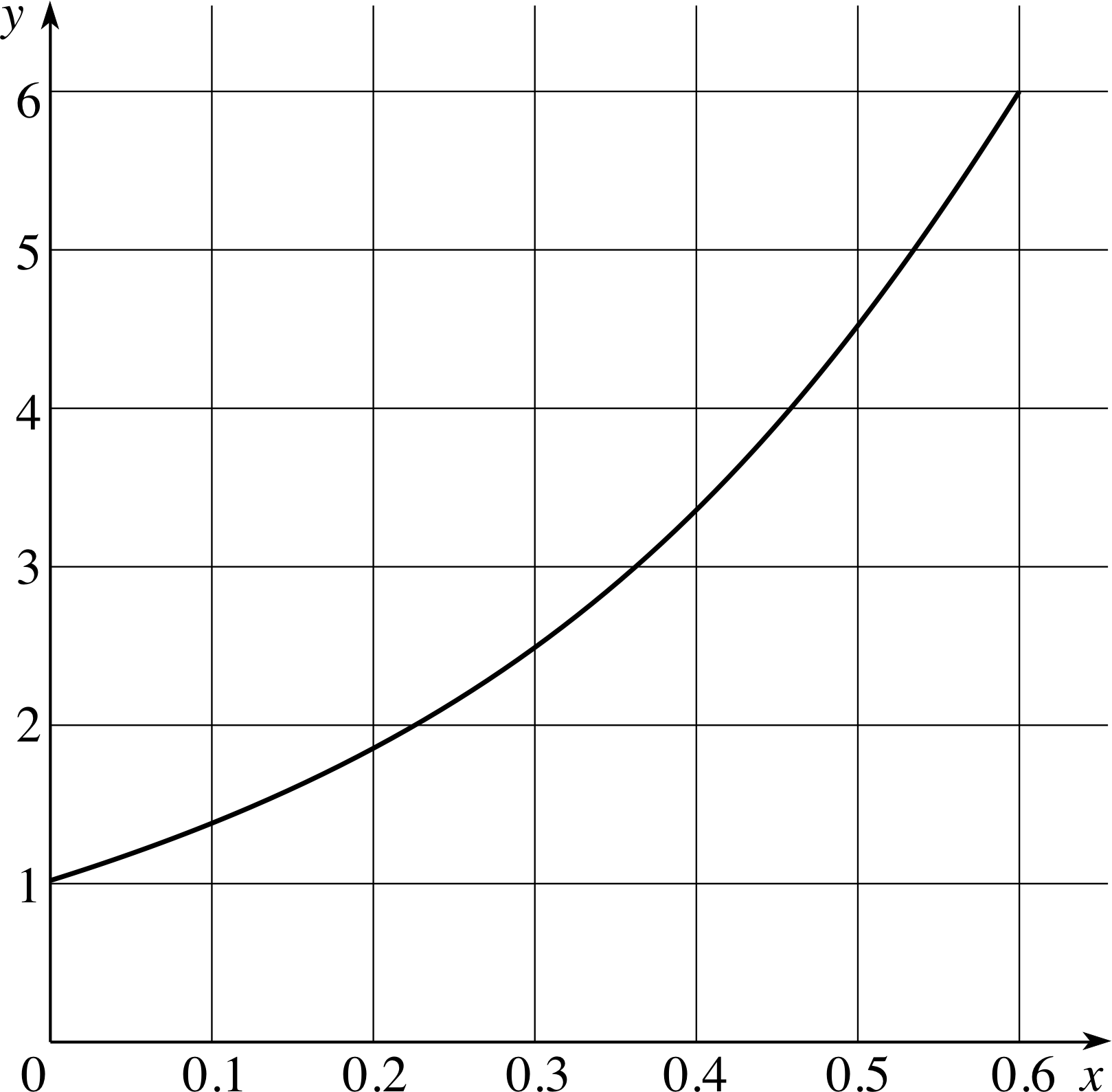
Figure 11 The graph of y (x) = exp(3x).
✦ Table 2 gives some values for the function y (x) = exp(3x). Figure 11 shows the graph of this function for the range x = 0 to x = 0.6. Draw tangents at the points y = 2 and y = 3 and measure their gradients. Suggest a relationship between the values of y and the gradient.
| x | exp(3x) |
|---|---|
| −1.0 | 0.050 |
| −0.5 | 0.223 |
| 0 | 1.000 |
| 0.5 | 4.482 |
| 1.0 | 20.086 |
| 1.5 | 90.017 |
| 2.0 | 403.429 |
✧ At any value of y, the gradient is 3y. Your measured values should have been close enough to the true values (6 and 9) to suggest this result.
You have just illustrated an important general rule about exponential functions:
For any function y (x) = exp(kx), the gradient at any value of x is ky (x), and so the rate of change ∆y/∆x = ky (x).
In other words, we seem to have found the function that satisfies the general condition for exponential change. So far, though, we have looked only at examples where k is positive (i.e. exponential growth), whereas we also need to be able to deal with exponential decay, where k is negative.
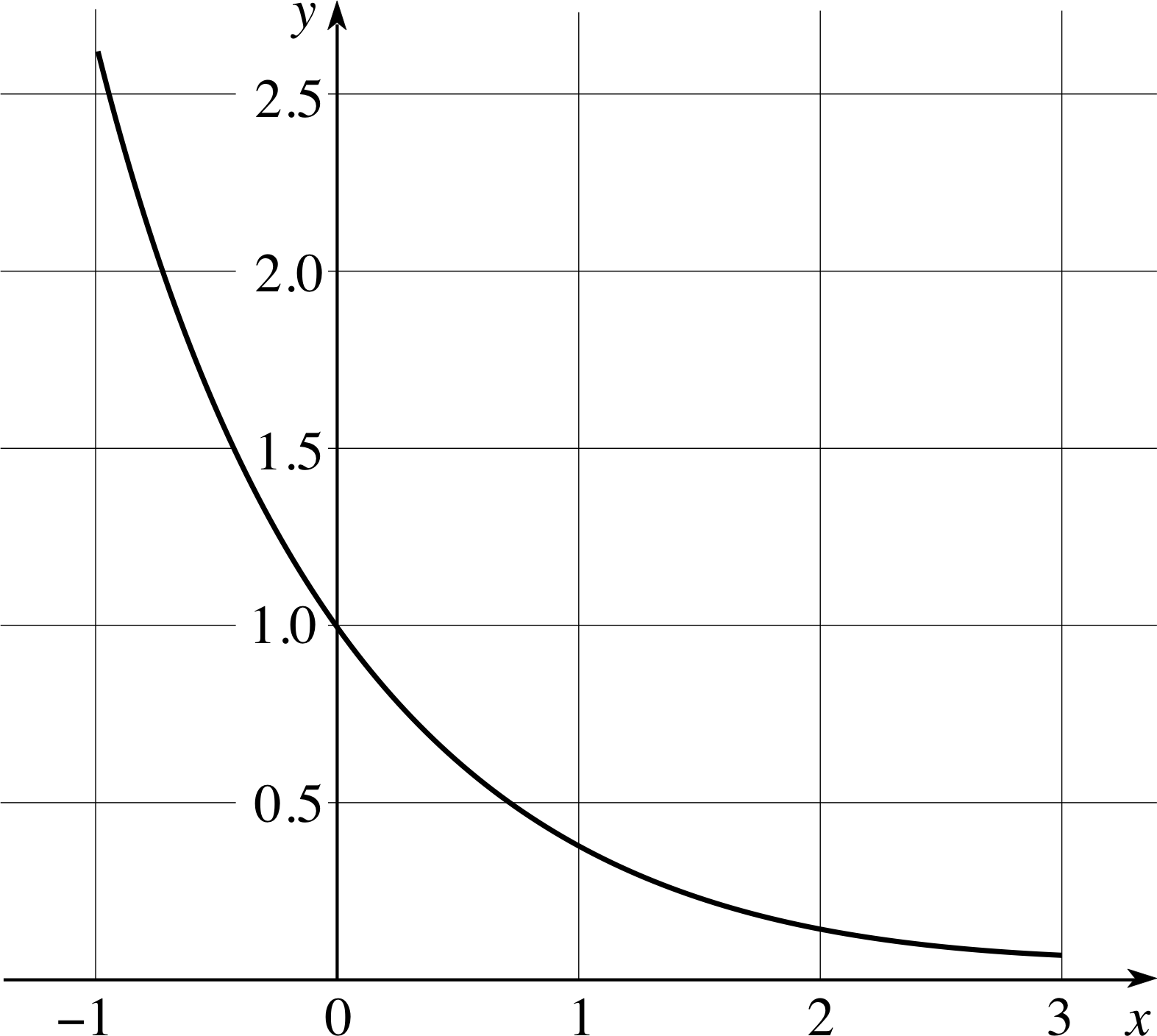
Figure 12 The graph of the function y (x) = exp(−x).
✦ Figure 12 shows a graph of the function y (x) = e−x (i.e. k = −1). What is the sign of the gradient at any point on the curve? What is the relationship between the gradient and the value of y?
(Draw tangents and measure their gradients if you have to, but you can probably guess the answer.)
✧ The gradients are all negative. At any value of x the gradient is −y (x).
The above example illustrates that the exponential function y (x) = exp(kx), with a suitable value of k, can describe both exponential growth and exponential decay. So we now have an almost complete description of any exponential change. Why ‘almost’? So far, we have neglected the initial value of y. If y = exp(kx), then when x = 0, y = 1. Clearly, this is not necessarily true in all physical situations. Also, since the start of Subsection 2.3 we have been treating x and y as a purely numerical variables, without any associated units. In practice we are certain to be interested in situations where y and x are physical quantities that involve units of measurement.
Dealing with these remaining conditions is actually very straightforward. All we have to do to represent a general exponential change is to use a function of the form y0 exp(kx). Thus:
For any exponential change, i.e. any change in which ∆y/∆x = ky
y (x) = y0 exp(kx)(8)
where y0 is the value of y when x = 0.
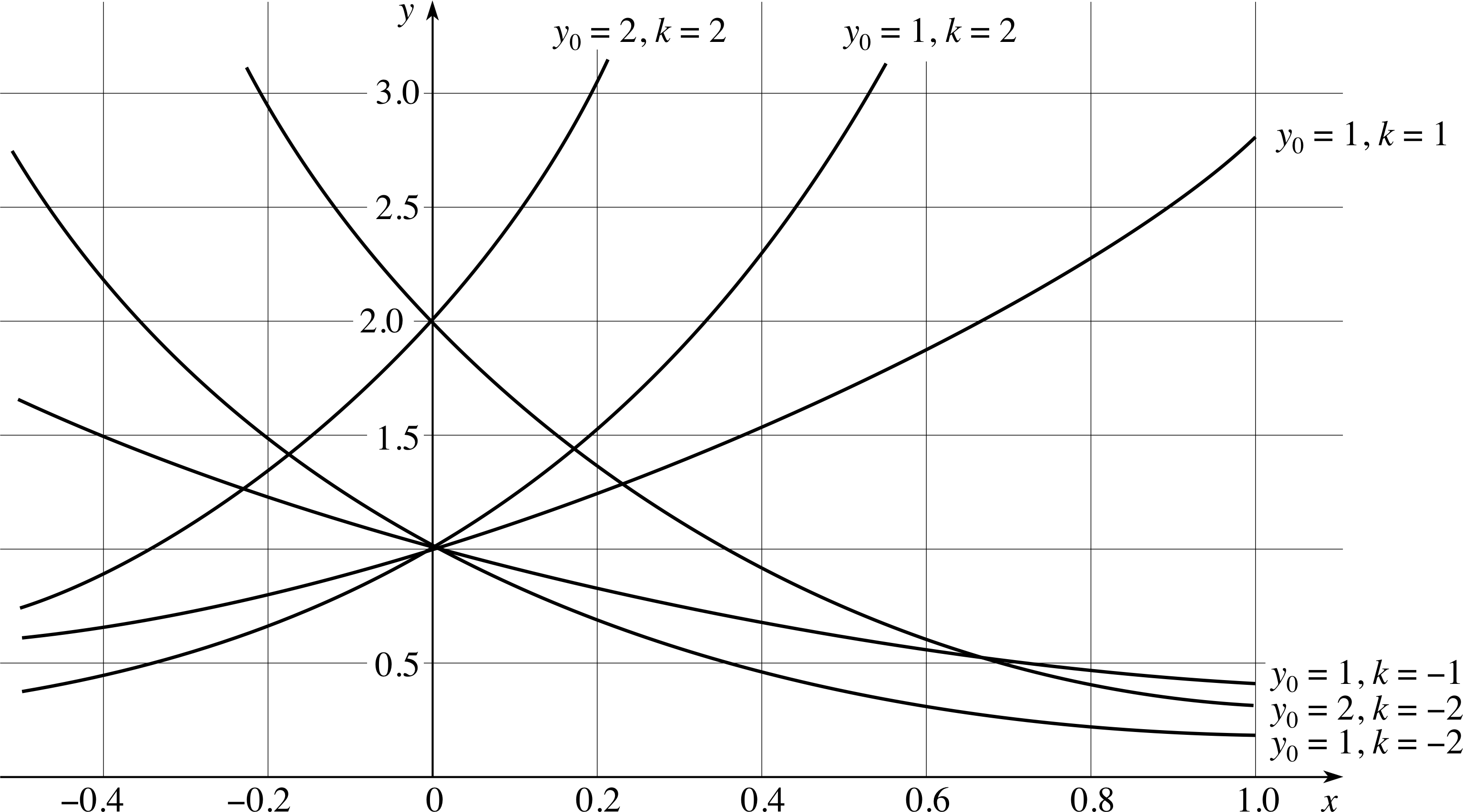
Figure 13 Graphs of the function y (x) = y0ekx for various values of y0 and k.
As far as units are concerned, y will have the same units as y0, and the product kt must be a pure number (i.e. dimensionless), so if x is a time in seconds, say, then the units of k should be seconds−1. i
Figure 13 shows the graphs of the exponential function y = y0ekx for various values of y0 and k. If you measured the gradients of tangents to any of these graphs you would find that in each case they satisfy the equation ∆y/∆x = ky at every value of x.
This illustrates the general rule that for exponential functions the initial value of y does not alter the relationship between the value of y and the gradient. So, we now have a complete ‘recipe’ for describing exponential change.
Question T7
When a capacitor discharges, ∆Q/∆t = −Q/(RC). If the initial charge is Q0, write an equation that describes how Q changes with time (i.e. write a definition of Q as a function of time).
Answer T7
k = −1/RC (see Answer T2) and so Q (t) = Q0 e−t/RC
Note that this could also be written as Q (t) = Q0 exp(−t/RC)
Question T8
Radioactive decay may be described by the equation N = N0ekt. What are the values of N0 and k for the decay shown in Figure 6?
Answer T8
N0 = 20 × 1010 (= 2 × 10¹¹). When N = 10 × 1010, the gradient ∆N/∆t = −5 × 10⁴ s−1, so
k = (∆N/∆t)/N = −5 × 10⁻⁷ s−1
We will now consider some specific examples of exponential change.
Half-lives and decay absorption coefficients
Apart from the proportionality between the function and the value of its gradient, y (t) = y0ekt has another interesting property. To see this, consider the effect of increasing t in a series of equal steps, say from 0 to 1/k, to 2/k, to 3/k, and so on. What are the corresponding values of y (t)? They are y0, y0e, y0e2, y0e3, and so on. Clearly, equal additions to t cause y (t) to change by equal multiplicative factors. This is true whatever the size of the additions to t may be (though different sized increments naturally correspond to different multiplicative factors), and it applies to exponential decay as well as exponential growth. In fact, the best known example of this is probably the use of half–life to characterize the decay of radioactive nuclei. Such decays are described by an exponential function of the form N (t) = N0e−λt, so in any time interval of length 1/λ the number of nuclei will decrease by a factor of e−1. Similarly, in any interval of length 0.693/λ the number of nuclei is reduced by a factor of 0.5. That’s why this is called the half-life. i
So far we have been concentrating on changes with time, but we have already noted that an exponential function is not limited to such changes. For example, when a parallel beam of electromagnetic radiation passes through matter, its intensity I i is related to the distance x that it has travelled through the medium by an exponential function: I = I0 exp(−μx) where μ is called the absorption coefficient. It also depends on the nature of the radiation and the nature of the matter. For every additional distance 1/μ that the beam travels through the matter, its intensity is reduced by a factor of e−1.
✦ What are the dimensions of μ?
✧ Since μx must be dimensionless μ must be reciprocal length, [L−1].
The function at
Throughout the last two subsections, we have been mainly concerned with functions of the form y (x) = y0ekx. But we have also seen that functions such as 2x and 3x also satisfy the requirement that their gradients are proportional to their values at any given value of x. Clearly then, the exponential function exp(x), or ex, is just one special example of the kind of function that can describe exponential change. More generally, any function of the type y (x) = y0a kx (where a is any positive number) will describe exponential change, though it will not satisfy the equation ∆y/∆x = ky. For instance, in Subsection 2.3, you saw that the gradient of the graph of y (x) = 2x is approximately ∆y/∆x ≈ 0.7y while that of y (x) = 3x is approximately ∆y/∆x ≈ 1.1y, so in both of these cases, where k = 1, it is certainly not the case that ∆y/∆x = ky even though ∆y/∆x is proportional to y. What really distinguishes the function y (x) = y0ekx is the fact that for it alone we can assert that ∆y/∆x = ky for all values of k.
Although the functions y (x) = y0ekx and y (x) = y0a kx are different (provided a ≠ e), there is a simple relationship between them. Because it is always possible to find a number c such that a = ec, for any positive value of a, it is always possible to write
y0a kx = y0(ec) kx = y0eckx (a > 0)
Thus, any function that describes exponential change can always be rewritten in terms of the exponential function, all we have to do is find the value of c that satisfies the equation a = ec. We will return to this in Subsection 3.2, where you will see how it is done.
A note on terminology In an expression such as q p (where p and q are either constants or variables), the power p is sometimes called the exponent of q. i Correspondingly, some authors use the term ‘exponential function’ to mean all functions of the type y (x) = a x. Those authors still use exp(x) to represent ex, but they sometimes call it the natural exponential function (since it arises from descriptions of naturally–occurring processes) in order to distinguish it from other functions of the type a x. However, in FLAP the term exponential function is generally used to mean a function of the form y (x) = ex or y (x) = ekx. Variables related by functions of the form y (x) = y0ekx are generally said to satisfy exponential laws. Such laws arise in many areas of physics.
2.5 Evaluating the number e
In Subsection 2.3, the value of e was produced more or less out of a hat, and was then shown to have the necessary properties to describe exponential change. Now we will show how the value of e can be calculated from first principles.
We start from the requirement that we want a number e such that if y (t) = y0ekt, then ∆y/∆t = ky. In order to avoid having to deal with negative numbers, we will consider an example of continuous exponential growth. Our original example of the growth of an investment is now not a very good one, since the interest is added only once a year and so the value goes up in steps rather than continuously. A better example would be the growth of a large population of organisms (aphids, perhaps, or bacteria) where the population changes over even a very short time interval.
Figure 14 An approximate graph of N against t where N0 = 105, k = 0.1 s−1 and (a) ∆t = 5 s, (b) ∆t = 1 s.
Suppose the number of organisms at time t is N (t), and that at any time t the instantaneous rate of change is ∆N/∆t = kN (t). Even if we do not have an expression for N (t) in terms of t, we can still use the given information to draw an approximate graph of N against t. To do this we note that the increase in the population over a small time interval ∆t will be approximately ∆N = kN (t)∆t. (This is only an approximation because the equation ∆N/∆t = kN (t) will not be completely accurate for any finite value of ∆t, no matter how small.)
So, if N0 is the number of organisms at the start of a time interval ∆t, the approximate number at the end of that interval will be N0 + ∆N = N0 + kN0∆t. This process can be repeated for the next interval ∆t, by taking N1 = N0 + kN0∆t as the new starting value and ∆N = kN1∆t as the increment over that second interval. This can be continued until we have built–up a complete (though approximate) graph of N (t) over any desired period of time.
Figure 14a shows such a graph for k = 0.1 s−1 and N0 = 105, drawn using a time interval of ∆t = 5 s. If a time interval of ∆t = 1 s were used (still with k = 0.1 s−1), then the graph would not only be smoother but it would also climb more steeply, as shown in Figure 14b. The increased steepness arises because, instead of using the same rate of change for a whole 5 s, based on the value of N at the start of that interval, we calculate a new rate of change after only 1 s, based on a slightly larger N.
✦ Which graph in Figure 14 is the better approximation to the real situation? How could the graphs be made even more realistic?
✧ Figure 14b is a better approximation because it follows the changes in N and ∆N/∆t more closely. The graphs can be made even more realistic by choosing a smaller time interval.
| t/s | (a) N/104 when ∆t = 5 s |
(b) N/104 when ∆t = 1 s |
||||
|---|---|---|---|---|---|---|
| 0 | 10.000 | 10.000 | ||||
| 1 | 11.000 | |||||
| 2 | 12.100 | |||||
| 3 | 13.310 | |||||
| 4 | 14.641 | |||||
| 5 | 15.000 | 16.105 | ||||
| 6 | 17.716 | |||||
| 7 | 19.487 | |||||
| 8 | 21.436 | |||||
| 9 | 23.579 | |||||
| 10 | 22.500 | 25.937 |
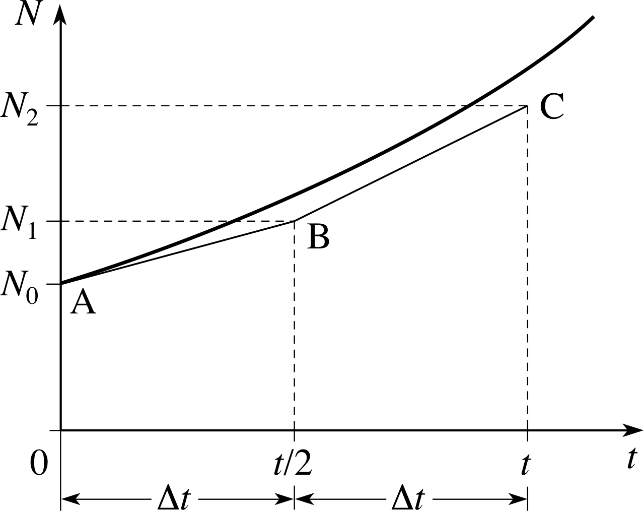
Figure 15 Estimating N (t) by dividing a the time t into small intervals. The curve represents the actual variation of N with t.
Table 3 shows the values used to plot Figure 14.
Let us now see what happens as we make ∆t smaller and smaller. Figure 15 illustrates the procedure. N0 is the initial number of organisms and t is some arbitrary period of time which can be subdivided into intervals. If we divide t into 2 equal intervals of length ∆t = t/2, and if N1 is the approximate number after the first interval of length t/2, then
$\displaystyle N_1=N_0+\frac{kN_0t}{2}=N_0\left(1+\frac{kt}{2}\right)$(9)
and after the second interval of length t/2
$\displaystyle N_2=N_1+\frac{kN_1t}{2}=N_1\left(1+\frac{kt}{2}\right)$(10)
Combining Equations 9 and 10, we find
$\displaystyle N_2=N_0\left(1+\frac{kt}{2}\right)^2$(11)
Now, if we had chosen to use 10 smaller intervals, each of length t/10, we would have obtained a somewhat different, and more accurate, estimate of the total number of organisms after time t:
$\displaystyle N_{10}=N_0\left(1+\frac{kt}{10}\right)^{10}$
Similarly, if we had used n equal intervals, then we would have found
$N_n = N_0\left(1+\dfrac{kt}{n}\right)^n$(12)
If we now let the value of n become larger and larger we can expect the value of N n to get closer and closer to the true final value (which we know to be N0ekt). Thus, as n becomes larger the following approximation becomes increasingly accurate:
$N_0e^{kt} = N_0\left(1+\dfrac{kt}{n}\right)^n$
For reasons that will soon become apparent, it is useful to eliminate n from this relationship in favour of a new variable m defined by m = n/kt. In making this substitution it is important to remember that the final power of n must be replaced by mkt, and the statement that the approximation becomes increasingly accurate as n becomes larger should also be restated in terms of m. Thus, as m becomes larger the following approximation becomes increasingly accurate:
$N_0e^{kt} = N_0\left(1+\dfrac{1}{m}\right)^{mkt} = N_0\left[\left(1+\dfrac{1}{m}\right)^m\right]^{kt}$(13)
It follows from Equation 13 that e ≈ (1 + 1/m) m, and that this approximation becomes increasingly accurate as m becomes larger and larger. This statement can be made more concise by using the mathematical idea of a limit. We say that e is the limit of (1 + 1/m) m as m tends to infinity. This is conventionally written as:
$\displaystyle e = \lim_{m\rightarrow\infty}(1 + 1/m)^m$(14) i
| m | a |
|---|---|
| 2 | 2.2500 |
| 5 | 2.4883 |
| 10 | 2.5937 |
| 102 | 2.7048 |
| 103 | |
| 104 | |
| 105 |
Question T9
Given that a = (1 + 1/m) m, complete Table 4 (using a calculator) and thus confirm that (1 + 1/m) m provides an increasingly good approximation to e as m becomes larger and larger.
| m | a |
|---|---|
| 2 | 2.2500 |
| 5 | 2.4883 |
| 10 | 2.5937 |
| 102 | 2.7048 |
| 103 | 2.7169 |
| 104 | 2.7181 |
| 105 | 2.7183 |
Answer T9
The completed table is given in Table 6.
3 Logarithmic functions
In Section 2, you saw how exponential changes can be described by a function of the general form y (t) = y0 exp(kt). Given values for y0 and k, this function provides a unique value of y for any given value of t. In this section our main aim is to investigate the inverse function, that tells us the value of t corresponding to any given value of y. However, we begin our investigation by examining a slightly different question: given that x = 10y, what is the value of y that corresponds to a given value of x? In other words, given that x = 10y, we want to know the inverse function that will enable us to write y as a function of x.
3.1 Logarithms to base 10: the inverse of 10x
For some values of x, we can find y such that x = 10y, without really thinking about inverse functions at all. For example, if x = 100 then, since 100 = 10 × 10 = 102, y must be equal to 2.
✦ If x = 10y, what is y when, (a) x = 10 000, and (b) x = 0.1?
✧ (a) 10 000 = 104, so y = 4
(b) 0.1 = 10−1, so y = −1
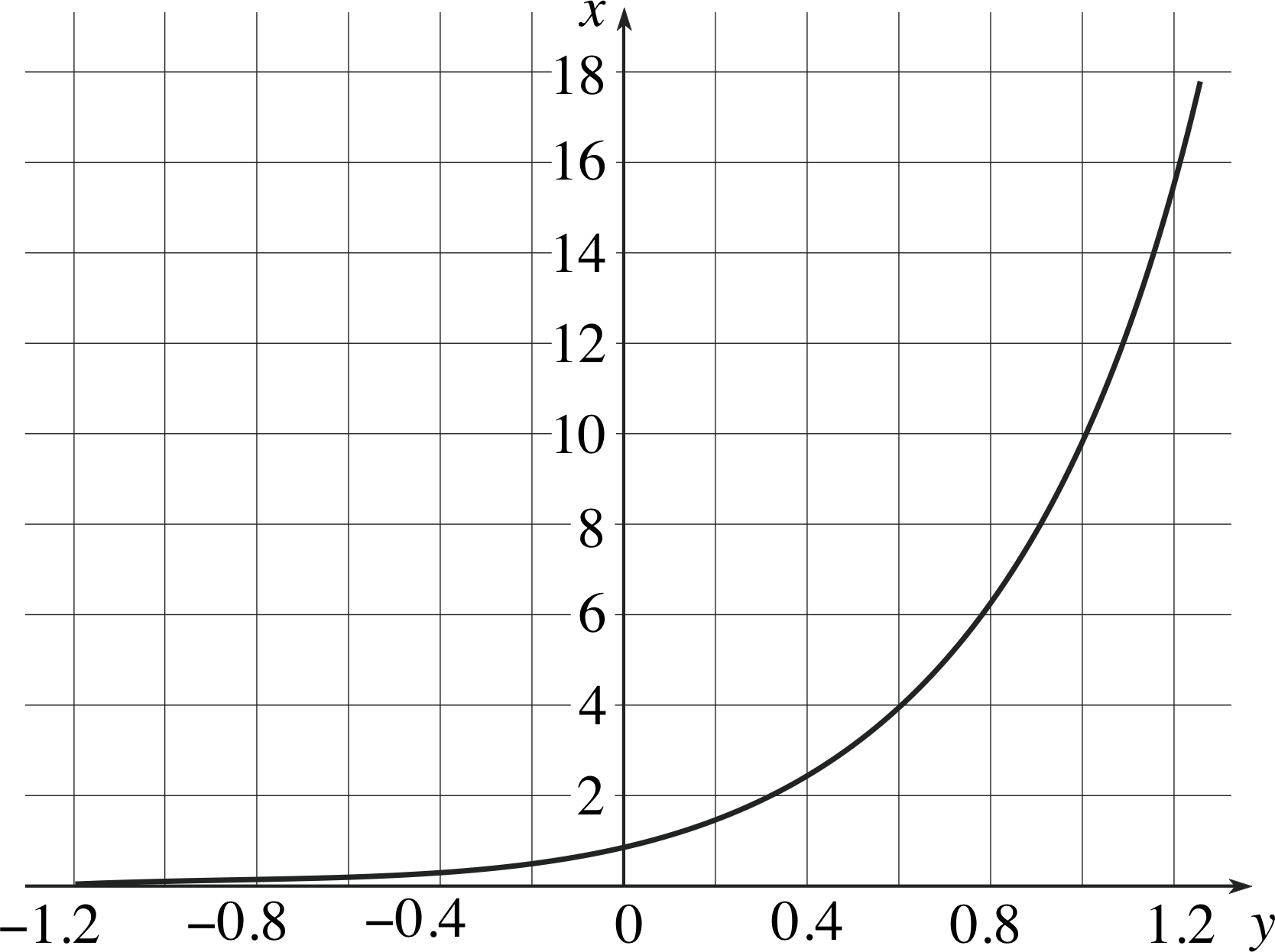
Figure 16a A graph of the function x = 10y with the x–axis vertical and the y–axis horizontal.
Figure 16a is a graph of the equation x = 10y, plotted with the x–axis vertical and the y–axis horizontal. This may look odd, but when plotting graphs it is conventional to plot values of the independent variable along the horizontal axis and values of the dependent variable along the vertical axis, and that is exactly what we have done. It is the choice of names for the variables that is unconventional in this case, not the graph plotting. In any event, it is clear from Figure 16a that each value of x corresponds to a different value of y, and that means it will be possible to define an inverse function to x = 10y. The graph of this inverse function (with conventional x– and y–axes orientation) is shown in Figure 16b. It was obtained by re–plotting the data from Figure 16a so as to show y as a function of x. (This process is equivalent to reflecting the curve in Figure 16a in an imaginary mirror placed along the line y = x). This shows that we can, in principle, find y for any positive value of x.
Figure 16b A graph of the inverse function, y = log10 (x), plotted on axes with the conventional orientation.
The function of x shown in Figure 16b is usually denoted by y = log10 (x) and its value for a given value of x is called the logarithm to base 10 of x, or the common logarithm of x. This is an example of a logarithmic function – you will meet others in Subsection 3.2. As you can see from Figure 16b, it is only defined for positive values of x.
The logarithm to base 10 of x is the number y which satisfies the equation x = 10y, i.e.
y = log10 (x)
In other words, log10 (x) is the power to which we must raise 10 to obtain x.
We have written x in brackets in log10(x), to emphasize that we are dealing with a function, but the brackets are often omitted in practice. Note, too, that log10(x) is sometimes written as log(x).
From our definition we see that:
log10 (10) = 1 since 101 = 10
log10 (1) = 0 since 100 = 1
$\log_{10}\left(\dfrac{1}{10}\right) = -1 \quad\text{since}\quad 10^{-1}= 1$
Question T10
Without using your calculator, work out the values of:
(a) log10 (100)
(b) log10 (1000)
(c) log10 (0.1)
(d) log10 (0.001)
(e) log10 (101/2)
(f) log10 (10)
(g) log10 (1)
(h) log10 (101.52)
Answer T10
(a) 100 = 102, so log10 (100) = 2
(b) 1000 = 103, so log10 (1000) = 3
(c) 0.1 = 10−1, so log10 (0.1) = −1
(d) 0.001 = 10−3, so log10 (0.001) = −3
(e) 101/2 = 100.5, so log10 (101/2) = 0.5
(f) 10 = 101, so log10 (10) = 1
(g) 1 = 100, so log10 (1) = 0
(h) log10 (101.52) = 1.52
✦ Use the x y key on your calculator to find 100.397 94 and 10−2.30 103, and hence find values for log10 (2.5) and log10 (0.005) to five decimal places.
✧ log10 (2.5) = 0.397 94 and log10 (0.005) = −2.301 03
The values of log10 (x) are harder to calculate directly when x is not an obvious power of 10. However, they can be read from graphs such as that in Figure 16b, or found using the ‘log’ key on a calculator. For example, to find log10 (3.7), key in 3.7 then press the ‘log’ function key – you should obtain the answer 0.568 201 7.
✦ Use your calculator to find log10 (100), log10 (10), log10 (1), log10 (0.001), log10 (2) and log10 (3.16).
✧ log10 (2) = 0.301, and you can check your other answers with the answer to Question T10. Notice that, to two decimal places, 3.16 = 101/2.
Question T11
Use the log function key on your calculator to find x when (a) 10x = 6.8, (b) 10x = 537 and (c) 10x = 0.34. (Give your answers to four significant figures.)
Answer T11
(a) If 10x = 6.8, then x = log10 (6.8) = 0.8325
(b) 10x = 537, x = log10 (537) = 2.730
(c) 10x = 0.34, x = log10 (0.34) = −0.4685
(All to four significant figures.)
Question T12
Use your calculator to find (a) log10 (4.725), (b) log10 (47.25) and (c) log10 (472.5).
Without further use of the calculator, find (d) log10 (4725) and (e) log10 (4.725 × 10⁷).
Answer T12
(a) log10 (4.725) = 0.6744
(b) log10 (47.25) = 1.6744
(c) log10 (472.5) = 2.6744.
(d) A pattern has emerged – namely log10 (4.725 × 10¹⁰) = n + log10 (4.725). Therefore log10 (4725) = 3.6744 and log10 (4.725 × 10⁷) = 7.6744.
(This pattern is discussed further in Subsection 3.3).
We have already established that taking the logarithm to base 10 ‘undoes’ the operation of raising 10 to a power (see part (e) of Question T10, for example). Likewise, raising 10 to a power ‘undoes’ the operation of finding the logarithm to base 10. This can be expressed another way. If we eliminate y from Equation 15 we find
10log10 (x) = x
thereforelog10 (10x) = x(16)
The function 10x is sometimes called the antilog or antilogarithmic function. Antilogs can be found on a calculator using the ‘inverse’ and ‘log’ function keys. i
✦ Use the function keys on your calculator to find antilog(x) for x = 2, x = −1, x = 0.397 94 and x = −2.301 03. Key in the number, then press ‘inv’ and ‘log’.
✧ antilog(2) = 100, antilog(−1) = 0.1, antilog(0.397 94) = 2.5, antilog(−2.301 03) = 0.005. Notice that you have seen some of these results before, in Question T10 and the subsequent seeded question.
3.2 Logarithms to base e and other bases
In Subsection 3.1, we looked at logarithms based on powers of 10. It is possible to use numbers other than 10 as the base for logarithms – in fact it is possible to have logarithms to any base a that is greater than zero:
The logarithm to base a of x is the number y such that x = a y.
In other words, the logarithm to base a of x is the power to which we must raise a to obtain x, i.e. if x = a y then
y = loga (x)(17)
Just as the functions 10x and log10 (x) are the inverse of each other, so the functions a x and loga (x) are the inverse of each other. This can be expressed by eliminating y from Equation 17 to obtain x = aloga (x), or alternatively by eliminating x to obtain y = loga (a y). Replacing y by x throughout the second of these results (which we are free to do since we can always rename a variable) we see that for any base a:
ifaloga (x) = x
then loga (a x) = x(18)
✦ Given that N/N0 = 2kT, find an expression for T.
[Hint: Start by taking appropriate logs of both sides of the given equation.] i
✧ Taking log2 of both sides, we find log2 (N/N0) = log2 (2kT) thus, from Equation 18, log2 (N/N0) = kT so, T = (1/k) log2 (N/N0)
The most widely–used logarithms and logarithmic functions are those based on powers of 10 or on powers of the number e.
The logarithm to base e of x is the number y such that x = ey, i.e.
ifx = ey
then y = loge (x)(19)
and hence
exp[loge (x)] = x
andloge [exp(x)] = x(20)
Since the number e arises from the description of naturally–occurring processes (radioactive decay), the logarithmic function based on powers of e is often known as the natural logarithm and loge (x) is sometimes denoted by ln(x). i Note that loge (x) can be found on a calculator, in the same way as finding log10(x), the key is usually marked loge (x) or ln(x). (You may have to press ‘inv’ followed by ‘ex’ if your calculator doesn’t have a ‘loge’ or ‘ln’ key.)
✦ Given that e = 2.718 (to three decimal places), use the y x key on a calculator to find e1.5041, and hence write down an approximate value for loge (4.5).
✧ e1.5041 = 4.500 (to three decimal places), so loge (4.5) ≈ 1.5041. You can check the answer by using the loge (x) key on a calculator.
Question T13
Without using your calculator, what are the values of loge (1) and loge (e)?
Answer T13
loge (1) = 0, since e0 = 1 (a0 = 1 for any value of a). loge (e) = 1, since e1 = e.
Question T14
Using your answers to Question T13, and the value of loge (10) found using your calculator, sketch an approximate graph of the function loge (x) on the same axes as a graph (such as that in Figure 16b) of log10 (x).
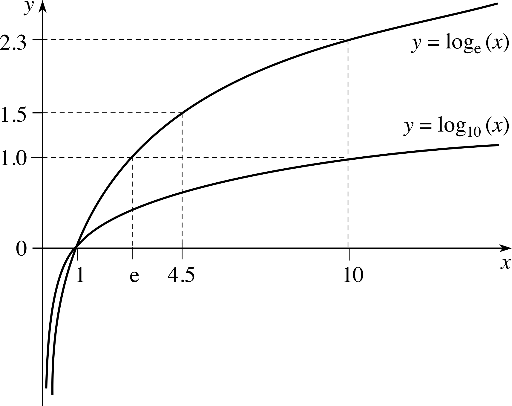
Figure 20 See Answer T14.
Answer T14
Figure 20 shows the graph of the function loge (x) drawn on the same axes as log10 (x). The graph of loge (10) is similar in shape to Figure 16b. Like log10 (x), it cuts the x–axis at x = 1. The rest of the curve can be estimated by drawing a curve through loge (10) ≈ 2.303, loge (e) = 1 (e ≈ 2.718) and loge (4.5) ≈ 1.5 (see the Seed Question above Question T13).
(The exact relationship between log10 (x) and loge (x) is discussed in Subsection 3.3).
Natural logarithms can, as you have just seen, be handled on a calculator in a similar way to common logarithms. Their inverse function, too, can be dealt with similarly. i
✦ Suggest how to find exp(x) on a calculator using the ‘inv’ (i.e. inverse) and ‘log’ keys. i Use this method to find e1.5041.
✧ Key in 1.5041, then press the inverse and loge function keys. You should obtain a value very close to 4.5.
We are now able to solve the problem posed at the start of Section 3 – namely, to write t as a function of y given that y (t) = y0 exp(kt). If we divide both sides of this equation by y0 we obtain y/y0 = exp(kt) = ekt. We can then use Equation 21 (or take loge of both sides) to deduce that:
ify = y0 exp(kt)
then loge (y/y0) = kt(21)
so that t = (1/k) loge (y/y0)
When dealing with exponential decay, the constant k will be negative, and care will need to be taken when dealing with signs. For example, when a capacitor discharges through a resistor, the charge Q on the capacitor is given as a function of time by Q = Q0 exp(−t/RC). To find the time at which Q reaches a certain value, divide both sides by Q0 to obtain Q/Q0 = exp(−t/RC), and then take loge of both sides to see that loge (Q/Q0) = −t/RC. So, t = −RC loge (Q/Q0).
We can also now solve the problem encountered at the end of Subsection 2.4, where we wanted to find a number c such that a kt = exp(ckt). In other words, since eckt = (ec) kt, we wanted to find the value of c such that a = ec. If we take loge of both sides of this equation we find c = loge (a). You will recall that this is an important result since it enables us to rewrite any function of the form y (t) = y0a kt in terms of the exponential function y (t) = y0eckt.
Question T15
Use your calculator to find x when:
(a) ex = 4.8 (b) ex = 10 (c) ex = 0.56
Answer T15
(a) ex = 4.8, x = loge (4.8) = 1.569 (b) ex = 10, x = loge (10) = 2.303 (c) ex = 0.56, x = loge (0.56) = −0.5798
(All to four significant figures.)
Question T16
The number of organisms, N, in a certain population increases exponentially: N = N0 exp(kt) where k = 0.02 h−1. If N0 = 1000, how long does it take for the population to double, i.e. what is t when N = 2000? Without doing any further calculation, write down the time taken for N to increase from 2000 to 4000.
Answer T16
N = N0 exp(kt). Dividing both sides by N0, and using the fact that N/N0 = 2, gives us 2 = exp(kt) so loge (2) = kt and hence t = loge (2)/k = 0.693/(0.02 h−1) = 34.7 h. This applies both when N0 = 1000 and N = 2000, and when N0 = 2000 and N = 4000 – the time for the population to double is independent of the initial number N0.
Question T17
In a sample of radioactive material, the number, N, of polonium nuclei decays exponentially: N = N0 exp(−λt) where λ = 0.0133 s−1. How long does it take for the number of polonium nuclei to halve?
Answer T17
N =N0 exp(−λt). Dividing both sides by N0, gives us N/N0 = exp(−λt) where N/N0 = 1/2 so that 1/2 = exp(−λt) and therefore (taking logs of both sides) we find loge (1/2) = −λt so that
t = [loge (1/2)]/(−λ) = 0.693/(0.0133 s−1) = 52.11 s
Question T18
By finding a suitable value of k, rewrite the function y (x) = 3x in the form y (x) = ekx. Check your answer by finding 3x and exp(kx) when x = 2.
Answer T18
ek = 3, so k = loge (3) ≈ 1.099 (to four significant figures). y = exp(1.099x). 32 = 9, and exp(1.099 × 2) ≈ 9.007 ≈ 9. (The agreement becomes even better if k is taken to more significant figures.)
3.3 Properties of logarithms
In this subsection we examine some further properties of logarithms that can be deduced from the relationships we have already discussed together with the rules for manipulating indices that were summarized in Equations 3 to 6.
Products and quotients
First, let us look at the result of multiplying two numbers together where each is expressed as 10 raised to a power. i Suppose that x = 10p and y = 10q. By definition then, log10 (x) = p and log10 (y) = q (see Equation 15).
Now,xy = 10p × 10q = 10p + q
solog10 (xy) = log10 (10p + q) = p + q = log10 (x) + log10 (y)
thuslog10 (xy) = log10 (x) + log10 (y)
Of course, instead of working to base 10, we could equally well have written x and y as powers of some other number a, and then taken logs to base a. If we had done so we would have found the following general result:
loga (xy) = loga (x) + loga (y)(22)
You can illustrate this rule with the aid of a calculator. For example, log10 (3) = 0.477, log10 (7) = 0.845 and log10 (21) = 1.322 (all to three decimal places), i.e. log10 (21) = log10 (3) + log10 (7).
✦ Confirm that loge (21) = loge (3) + loge (7).
✧ loge (3) = 1.099, loge (7) = 1.946, loge (21) = 3.045 (= 1.099 + 1.946).
You have in fact already met another example of this rule. In Question T12, you saw that log10 (4.725 × 10n) = n + log10 (4.725) – which follows from Equation 22 because log10 (10n) = n. The next example demonstrates some properties of logs of quotients and reciprocals. i
✦ (a) By writing x = 10p and y = 10q, find an expression for log10 (x/y) in terms of log10 (x) and log10 (y).
(b) Use your answer to express log10 1(1/x) in terms of log10 (x).
✧ (a) log10 (x/y) = log10 (10p−q) = p − q = log10 (x) − log10 ( y).
(b) It follows that log10 (1/x) = log10 (1) − log10 (x). But, log10 (1) = 0. So, log10 (1/x) = −log10 (x).
The example above suggests the following general rules, which apply to logs to any base a:
loga (x/y) = loga (x) − loga (y)(23)
loga (1/x) = −loga (x)(24)
✦ Check Equations 23 and 24 with the aid of your calculator. For example, try x = 24, y = 8, using (a) logs to base 10, and (b) logs to base e.
✧ (a) log10 (24) = 1.380, log10 (8) = 0.903; log10 (3) = 0.477 = log10 (24) − log10(8) log10 (1/24) = log10 (0.0417) = −1.380 = −log10 (24).
(b) loge (24) = 3.178, loge (8) = 2.079; loge (3) = 1.099 = loge (24) −loge (8) loge (1/24) = loge (0.0417) = −3.178 = −loge (24).
Powers and roots
Suppose we have some number y = x n where n is an integer, then
$y = \underbrace{x \times x \times x \dots \times x}_{\color{purple}{\large{n\text{ factors}}}}$
It follows from Equation 24 that
$\log_a(y) = \underbrace{\log_a(x)+\log_a(x)+\dots+\log_a(x)}_{\color{purple}{\large{n\text{ terms}}}}$ i
thus, loga (x n) = n loga (x).
This is indicative of a more general result that applies to any power of x, not just integer powers:
loga (x b) = b loga (x)(25)
You can check Equation 25 with the aid of a calculator. For example, you can show that log10 (32) = log10 (9) = 2 log10 (3); that log10 (491/2) = log10 (7) = [log10 (49)]/2 and that log10 (41.73) = log10 (11.004) = 1.73 × log10 (4). i
✦ By taking logs to base 10 of both sides of the equation, find the value of x when 2x = 3 × 5x.
✧ x log10 (2) = log10 (3) + x log10 (5). So x [log10 (2) − log10(5)] = log10(3), and hence x log10(2/5) = log10(3), x = log10(3)/log10(2/5) = −1.199.
loga (xy) = loga (x) + loga (y)(Eqn 22)
loga (x/y) = loga (x) − loga (y)(Eqn 23)
loga (1/x) = −loga (x)(Eqn 24)
As you will see in Subsection 3.4, Equations 22 to 25 enable logs to be used in tackling a wide variety of problems in physics. But before we end this subsection, we will extend our discussion and show how to convert between different bases for logarithmic functions.
Changing the base of logarithms
In Subsection 3.2 we derived the following expression involving loga (x):
aloga (x) = x(Eqn 18)
Now suppose we take logs to another base, b, of both sides:
logb(aloga (x)) = logb(x)(26)
loga (x b) = b loga (x)(Eqn 25)
From Equation 25,
loga (x) × logb (a) = logb (x)(27)
So we have a relationship between the log of x to two different bases – most usefully, it enables us to convert between the two most widely–used bases:
log10 (x) × loge (10) = loge (x)(28) i
To three decimal places, loge (10) = 2.303, and so loge (x) = 2.303 × log10 (x). Using your calculator, you can verify that Equation 28 describes the relationships between loge (x) and log10 (x) for various values of x. But if you look at the answer to Question T14 you will see that the graph of loge (x) can be obtained from the graph of log10 (x) by re–scaling the y–axis by a factor of loge (10), just as Equation 28 implies.
Question T19
Use logs to base ten to find the value of x when 6 = 2x.
Answer T19
log10 (6) = x log10 (2), so x = log10 (6)/log10 (2) ≈ 2.585.
Question T20
By finding log10 (5) and log10 (2) on a calculator, calculate log2 (5).
Answer T20
From Equation 27, with b = 10, a = 2 and x = 5:
log10 (5) × log10 (2) = log10 (5)
and solog2 (5) = log10 (5)/log10 (2) ≈ 2.322
3.4 Using logarithms in physics
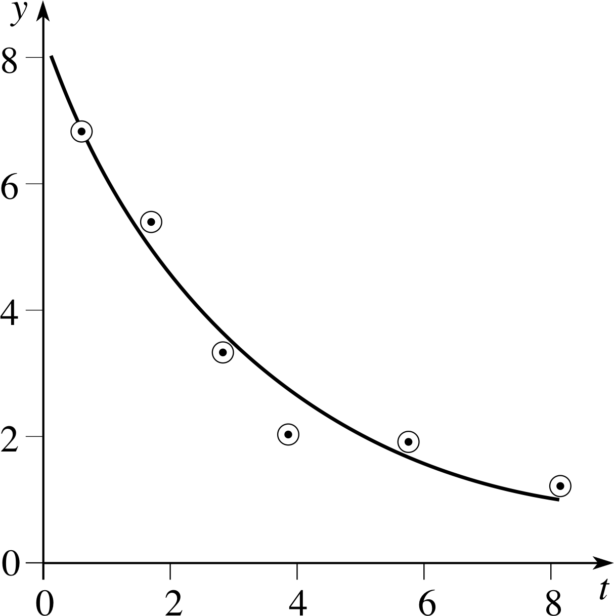
Figure 17 Experimental measurements of a quantity y that varies with time.
We have already seen one use of logarithms in physics – given that y = y0 exp(kt) we can find t in terms of y, i.e. t = [loge (y/y0)]/k. (See Subsection 3.2, in particular Questions T16 and T17). Now consider another problem related to exponential change. Suppose an experiment gives the results shown in Figure 17. Does this graph follow an exponential law? And if so, what is the value of k? It is hard to see whether or not Figure 17 really does represent an exponential function – you can measure gradients at various points, as we did in Subsection 2.2 (e.g. in Question T4), but this is time-consuming, and there are always uncertainties involved with drawing tangents. Let us consider an easier approach. If y does follow an exponential law, we must have y = y0 exp(kt), and hence
loge (y/y0) = kt(Eqn 21)
We can use Equation 23,
loga (x/y) = loga (x) − loga (y)(Eqn 23)
to write loge (y) − loge (y0) = kt, and hence
loge (y) = kt + loge (y0)(29)
If we recognize loge (y) as a simple variable (call it Y if you like) then we see that Equation 29 has the general form of the equation of a straight line (y = mx + c), so if we plot loge (y) against t, we should expect to get a straight line with gradient k that intersects the vertical axis at loge (y0). If the results do not follow an exponential law, the graph will not be a straight line. i
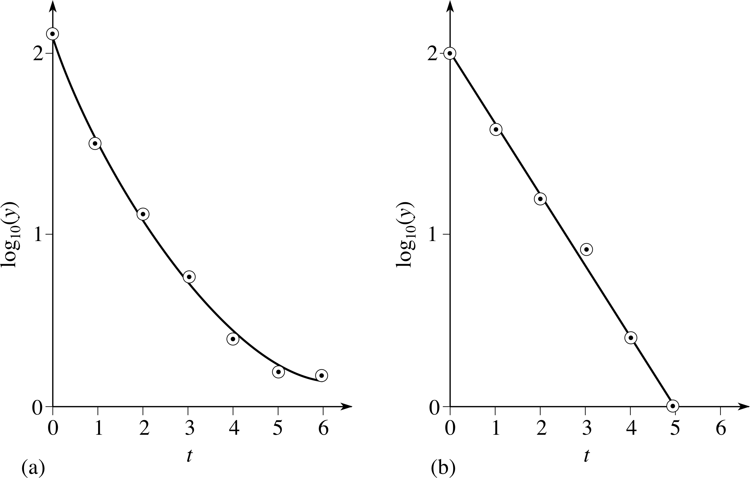
Figure 18 See Question T21.
Question T21
Figure 18 shows graphs of the results from two (hypothetical) experiments. Which graph shows that the relationship between y and t follows an exponential law, and what is the value of k in that case?
Answer T21
Figure 18b shows exponential decay, since the graph of log10 (y) plotted against t is a straight line. The gradient of this graph is −2/5 = −0.4. Thus the exponential law is y = y0 e−0.4t.
Similar techniques can be used for variables that obey a power law, i.e. a relation of the form y = kx p (or y = kt p) where the power, p, is some constant number. For example, suppose you think that variables F and r might obey a power law of the form
$\displaystyle F=\frac{k}{r^2}$(30) i
where k is an unknown constant. How can you test your hypothesis experimentally? And how can you find the value of k? The properties of logarithms, as summarized in Equations 2 – 5, provide a way. First, write the expression F = k/r2 in terms of log10 (F) and log10 (r), using Equation 23:
loga (x/y) = loga (x) − loga (y)(Eqn 23)
$\log_{10}(F) = \log_{10}\left(\dfrac{k}{r^2}\right) = \log_{10}{k}-\log_{10}(r^2)$(31)
Then, using Equation 25,
loga (x b) = b loga (x)(Eqn 25)
we find:log10 (F) = −2 log10 (r) + log10 (k)(32) i
✦ Suppose you were to plot a graph of log10 (F) against log10 (r). What would be its gradient and its intercept i on the vertical axis?
✧ Equation 32 is an equation of the form y = mx + c, so the gradient would be −2 and the intercept log10 (k).
Plotting a graph using logarithms thus enables you: to test the data to see whether they follow the expected exponential law, and to find the value of the constant k. Note that you do not have to use logs to base 10, since Equations 2 – 5 apply to logs to any base a. This technique can be summarized as follows:
ify = kx
thenloga (y) = p loga (x) + loga (k)(33)
so a graph of loga (y) against loga (x) has gradient p and intercept loga (k). The logs may have any base, though bases 10 or e are generally used.
Question T22
According to one of Kepler’s laws of planetary motion i, the orbital period, T, of a planet is related to its (average) distance, R, from the Sun: T2 = kR3. What would be the gradient of a graph of log10 (T) against log10 (R)? What would be the gradient if log to base e was used rather than base 10?
Answer T22
Taking log10 of both sides gives us
2 log10 (T) = log10 (k) + 3 log10 (R)
solog10 (T) = 3 log10 (R)/2 + log10 (k)/2
The gradient would be 3/2, irrespective of the base of the logs, since Equations 22 − 25 apply to logs to any base.
Question T23
An experimenter measures the period of oscillation, T, of various masses m supported by a spring and suggests, on theoretical grounds, that $T \propto \sqrt{m\os}$. How could the experimental data be tested to see whether $T \propto \sqrt{m\os}$ ?
Answer T23
If $T = k\sqrt{m\os}$, then $\log_{10}(T) = \log_{10}(k) + \log_{10}\left(\sqrt{m\os}\right) = \left.\log_{10}(k) + \left[log_{10}(m)\right]\middle/2\right.$, so a graph of log10 (T) against log10 (m) would have gradient 1/2.
(Note that logs to any base could be used and the gradient would still be the same.)
4 Closing items
4.1 Module summary
- 1
-
If the graph of some function y (t) is a straight line, then the Subsection 2.2rate of change of y is constant, and is equal to the Subsection 2.2gradient of the graph. If the graph is a curve, then the rate of change at any point is defined by the gradient of the tangent to the curve at that point.
- 2
-
If the rate of change of a variable is always proportional to the current value of that variable, then we can say that variable changes Subsection 2.3exponentially. If we represent the variable by y, and its rate of change by ∆y/∆t, we can write ∆y/∆t = ky, where a positive value of k characterizes exponential growth, and a negative value of k characterises exponential decay.
- 3
-
If ∆y/∆t = ky, then y (t) = y0 exp(kt), where the Section 2exponential function exp(kt) = ekt. The units of k are such that kt is a dimensionless quantity.
- 4
-
The following relationships are a consequence of the general properties of powers:
exey = ex+y
(ex) y = exy
${\rm e}^{-x} = \dfrac{1}{{\rm e}^x}$
${\rm e}^{x/y} = ({\rm e}^{1/y})^x$
- 5
-
Exponential functions are not restricted to describing changes with time. For example, the function exp(kx) (with k such that kx is dimensionless) could describe how a quantity varies with position or any other quantity.
- 6
-
The constant, e, is given in terms of a limit by:
$\displaystyle {\rm e} = \lim_{m \rightarrow\infty}(1 + 1/m)^m = 2.718$ (to three decimal places)
- 7
-
The logarithm to base a of x is the power to which we must raise a to obtain x. So, if x = a y, then
y = loga (x). The function loga (x) is thus the Section 3inverse of the function a x, hence aloga (x) = x and loga (a x) = x.
- 8
-
The most widely–used Section 3logarithmic functions have a = 10 and a = e.
- 9
-
Any function a x can be written in terms of the exponential function: a x = exp(cx), where c = loge (a).
- 10
-
The following relationships arise from the definition of a logarithmic function and the rules for combining indices:
loga (xy) = loga (x) + loga (y)(Eqn 22)
loga (x/y) = loga (x) − loga (y)(Eqn 23)
loga (1/x) = −loga (x)(Eqn 24)
loga (x b) = b loga (x)(Eqn 25)
- 11
-
The base (a or b) of any logarithmic function can be changed using the relationship
loga (x) × logb (a) = logb (x)(Eqn 27)
Sologa (x) = loge (x)/c, where c = loge (a).
- 12
-
If y = y0 exp(kt), then loge (y) = loge (y0) + kt, and a graph of loge (y) against t has gradient k and intercept loge (y0).
- 13
-
If y and x are related via a power law, y = kx p, then loga (y) = p loga (x) + loga (k) (Eqn 33) and a graph of loga (y) against loga (x) has gradient p and intercept loga (k).
4.2 Achievements
Having completed this module, you should be able to:
- A1
-
Define the terms that are emboldened and flagged in the margins of the module.
- A2
-
Recognize examples of exponential change.
- A3
-
Estimate the gradient at a point on a curved graph by drawing a tangent.
- A4
-
Sketch a graph of y = y0 exp(kt) and describe its significant features.
- A5
-
Write down an expression for the rate of change of y, where y = y0 exp(kt), for any given value of t or y.
- A6
-
Recognize and interpret the common expression for the number e written in terms of a limit.
- A7
-
Explain the relationships between the functions loga (x), a x and antilog(x) and know that many common applications of such functions use a = e or a = 10.
- A8
-
Sketch graphs of y = loge x and y = log10 x and describe their significant features.
- A9
-
Find the value of c such that a t = ect.
- A10
-
Manipulate and simplify expressions involving logarithmic and exponential functions of products, quotients and powers.
- A11
-
Change the base of a logarithmic function and find the value of c such that loga (x) = loge (x)/c.
- A12
-
Use a calculator to evaluate exponential functions, and logarithmic functions in base e and base 10.
- A13
-
Use logarithmic functions to test whether experimental data obey an exponential law or a power law, and to find the values of unknown constants in such relationships.
Study comment You may now wish to take the Exit test for this module which tests these Achievements. If you prefer to study the module further before taking this test then return to the Module contents to review some of the topics.
4.3 Exit test
Study comment Having completed this module, you should be able to answer the following questions, each of which tests one or more of the Achievements.
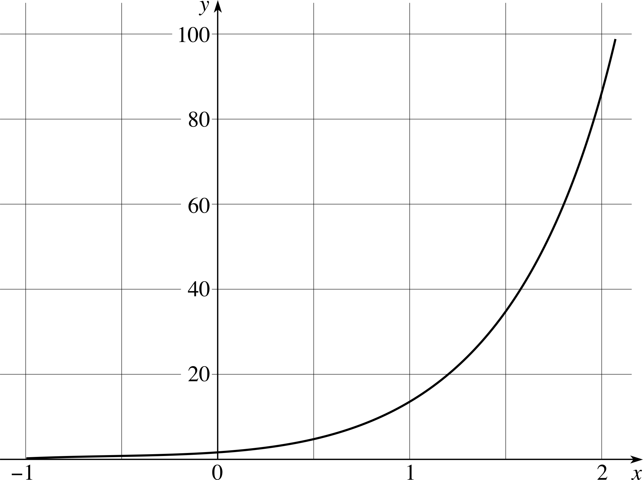
Figure 19 See Question E1.
Question E1 (A2 and A3)
Figure 19 shows how a certain variable y changes with x. By drawing tangents, estimate the gradient ∆y/∆x at y = 20, y = 40 and y = 60.
Are your answers consistent with y being an exponential function of x?
Answer E1
The measured gradients are approximately 45, 90 and 135 (the exact values depend on how you draw the tangents). These results are consistent with y being an exponential function of x, since the gradient is proportional to y (∆y/∆x ≈ 2.25y).
(Reread Subsection 2.1Subsections 2.1 and Subsection 2.22.2 if you had difficulty with this question.)
Question E2 (A4, A5 and A11)
For the function y = y0 exp(kt) with y0 = 3 and k = 0.1, (a) state a general expression for the gradient of the graph at any value of t, (b) calculate the gradient of the graph when t = 0 and when t = 2, and (c) sketch a graph of the function.
Answer E2
(a) Gradient ∆y/∆t = ky = ky0 exp(kt) = 0.3 exp(0.1t).
(b) When t = 0, ∆y/∆t = ky0 = 0.3; when t = 2, ∆y/∆t = 0.3 exp(0.2) ≈ 0.3664.
(c) Your sketch should resemble Figure 10, with the curve intercepting the y–axis at y = 3.
(Reread Subsection 2.3Subsections 2.3 and Subsection 2.42.4 if you had difficulty with this question.)
Question E3 (A9)
Rewrite the equation y = 10bx in terms of the exponential function exp(x).
Answer E3
We need a number k such that 10bx = ekx, i.e. 10b = ek. If we take loge of both sides, we find b loge (10) = k, so y = exp[bx loge (10)].
(Reread Subsection 3.2 if you had difficulty with this question.)
Question E4 (A10)
Given that log10 (3) = 0.477 and log10 (2) = 0.301, evaluate the following without using a calculator:
(a) log10 (300), (b) log10 (6), (c) log10 (60)
Answer E4
(a) log10 (300) = log10 (3 × 100) = log10 (3) + log10 (100) and log10 (100) = 2, therefore log10 (300) = 0.477 + 2 = 2.477.
(b) log10 (6) = log10 (3 × 2) = log10 (3) + log10 (2), therefore log10 (6) = 0.477 + 0.301 = 0.778. (c) log10 (60) = log(6 × 10) = log(6) + log(10) and log(10) = 1, therefore log10 (60) = 0.778 + 1 = 1.778.
(Reread Subsection 3.1Subsections 3.1 and Subsection 3.33.3 if you had difficulty with this question.)
Question E5 (A7 and A10)
Without using your calculator, simplify:
(a) exp[loge (π)], (b) loge (eπ) (c) $\log_{\pi}\left(\pi^{\sqrt{2\os}}\right)$
Answer E5
(a) exp[loge (π)] = π (b) loge (eπ) = π (c) $\log_{\pi}\left(\pi^{\sqrt{2\os}}\right) = \sqrt{2\os}$
(Reread Subsection 3.1Subsections 3.1, Subsection 3.23.2 and Subsection 3.33.3 if you had difficulty with this question.)
Question E6 (A11 and A12)
Find loge (π) and loge (2) on your calculator and hence evaluate log2(π).
Answer E6
$\log_2(\pi) = \dfrac{\log_{\rm e}(\pi)}{\log_{\rm 2}(2)} = \dfrac{1.145}{0.693} = 1.65
(Reread Subsection 3.3 if you had difficulty with this question.)
| A | T |
|---|---|
| 1 | 0.70 |
| 3 | 1.46 |
| 6 | 2.31 |
| 10 | 3.25 |
| 20 | 5.16 |
| 30 | 6.76 |
| 45 | 8.86 |
Question E7 (A12 and A13)
The results of an (hypothetical) experiment are given in Table 5. Suppose the data obey a law of the form T = kAα. Find k and α by plotting a suitable graph.
| A | T | log10 (A) | log10 (T) |
|---|---|---|---|
| 1 | 0.70 | 0.00 | −0.155 |
| 3 | 1.46 | 0.48 | 0.164 |
| 6 | 2.31 | 0.79 | 0.364 |
| 10 | 3.25 | 1.00 | 0.512 |
| 20 | 5.16 | 1.30 | 0.713 |
| 30 | 6.76 | 1.48 | 0.830 |
| 45 | 8.86 | 1.65 | 0.948 |
Answer E7
Taking logs to base 10 of both sides of this equation we get log10 (T) = log10 (k) + α log10 (A). The values are given in Table 7. This is a straight line of the form y = mx + c, therefore if log10 (T) is plotted against log10 (A) (as in Figure 21), the intercept on the vertical axis will give us log10 (k) = −0.16 so k = 0.7, and the gradient gives us α ≈ 0.67. (You could plot loge (T) against loge (A), which would give a straight line with the same gradient α, but the intercept would be (k) = −0.36, giving k = 0.7 as before.)
(Reread Subsection 3.3Subsections 3.3 and Subsection 3.43.4 if you had A difficulty with this question.)
Figure 21 See Answer E7.
Study comment This is the final Exit test question. When you have completed the Exit test go back and try the Subsection 1.2Fast track questions if you have not already done so.
If you have completed both the Fast track questions and the Exit test, then you have finished the module and may leave it here.
Study comment Having read the introduction you may feel that you are already familiar with the material covered by this module and that you do not need to study it. If so, try the following Fast track questions. If not, proceed directly to the Subsection 1.3Ready to study? Subsection.