MATH 1.3: Functions and graphs |
PPLATO @ | |||||
PPLATO / FLAP (Flexible Learning Approach To Physics) |
||||||
|
1 Opening items
1.1 Module introduction
What are functions? Dictionaries give the following definitions:
Function Math a variable quantity regarded in relation to other(s) in terms of which it may be expressed or on which its value depends. (one of four meanings)
Concise Oxford Dictionary, 8th Edition (1990–) Oxford University Press.
Function (math) a relation that associates with every ordered set of numbers (x, y, z ...) a number f (x, y, z ...) for all the permitted values of x, y, z ... (one of six meanings)
Longmans English Larousse, (1968–) Longmans.
Not very helpful, you may think. If the dictionaries cannot say anything clearer than that, how will you understand? Of course the purpose of a dictionary is to define rather than explain.
This module is a first step into applicable mathematics beyond the most elementary arithmetic and algebra. The idea of a function is a very wide one, wider than we shall need to deal with. In this module we shall see how functions are used, and how they should be looked at, thought about and described.
One very useful way of looking at and thinking about a function is to use its graph; this is a pictorial representation of the function, and shows a substantial part of its behaviour at once. We shall devote a good deal of time in this module to the study of graphs and how to draw them.
Subsection 2.1 of this module defines and explains the concept of a function in very general terms. Subsection 2.2Subsections 2.2 and Subsection 2.32.3 examine functions from a more mathematical point of view and introduce the terminology and notation used to describe them. The rest of the module is mainly concerned with the representation of functions. Subsection 2.4 deals with representation by tables and equations, and the whole of Section 3 is devoted to the important topic of graphical representation. Subsection 3.1Subsections 3.1 to Subsection 3.33.3 are concerned with the principles and conventions of graph drawing, while Subsection 3.4Subsections 3.4 to Subsection 3.73.7 present a catalogue of polynomial functions and also cover related matters such as the analysis of straight-line graphs, the nature of (local) maxima, (local) minima and points of inflection, and the behaviour of reciprocal functions. Section 4 deals briefly with the more advanced topics of inverse functions and functions of functions.
Study comment Having read the introduction you may feel that you are already familiar with the material covered by this module and that you do not need to study it. If so, try the following Fast track questions. If not, proceed directly to the Subsection 1.3Ready to study? Subsection.
1.2 Fast track questions
Study comment Can you answer the following Fast track questions? If you answer the questions successfully you need only glance through the module before looking at the Subsection 5.1Module summary and the Subsection 5.2Achievements. If you are sure that you can meet each of these achievements, try the Subsection 5.3Exit test. If you have difficulty with only one or two of the questions you should follow the guidance given in the answers and read the relevant parts of the module. However, if you have difficulty with more than two of the Exit questions you are strongly advised to study the whole module.
Question F1
Sketch a graph of the function f (x) = x3 − 4x where x is any real number.
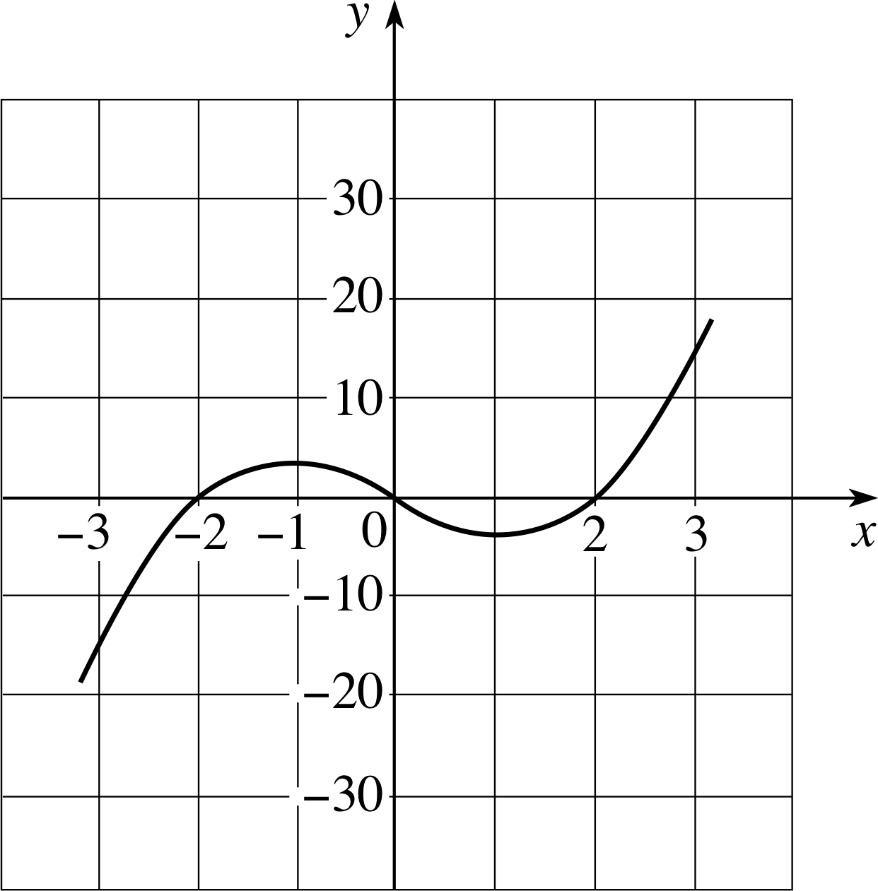
Figure 9 The graph of the function f (x) = x2 − 4x.
Answer F1
See Figure 9.
Question F2
If H (x) = x2 − 4x + 6, where x is any real number, rewrite H (x) in completed square form and hence find the coordinates of the vertex. Does the graph of H (x) intersect the x–axis? If so, where is the intersection located? Does H (x) have an inverse function?
Answer F2
H (x) = x2 − 4x + 6 = x2 − 4x + 4 + 2 = (x − 2)2 + 2
This last expression is the completed square form. The vertex is situated at the point (2, 2). The graph does not intersect the x–axis, because the discriminant b2 − 4ac is negative. H (x) does not have an inverse function because its graph is a parabola, so different values of x do not necessarily correspond to different values of H (x).
Question F3
Find the asymptotes of the graph of the function
g (x) = (x − 2)2/(x − 1) where x ≠ 1
Answer F3
As x approaches 1 from above (i.e. decreasing from even greater values of x), g (x) becomes a larger and larger positive number. As x approaches 1 from below (i.e. from lower values of x), g (x) becomes a larger and larger negative number. Thus x = 1 is an asymptote. When x is a large number, positive or negative, g (x) ≈ x2/x = x. Thus the line y = x is also an asymptote. These are the only asymptotes, as you can confirm by sketching the graph.
1.3 Ready to study?
Study comment In order to study this module you will need to understand the following terms: element (of a set), equation, fraction, inequality, integer, modulus, power_mathematicalpowers, real number, reciprocal, set, roots. If you are uncertain about any of these terms you can review them now by referring to the Glossary, which will indicate where in FLAP they are developed. In addition, you will need to be familiar with SI units, and be able to expand, simplify and evaluate algebraic expressions that involve brackets. If you are uncertain about your ability to perform these operations, you should again refer to the Glossary for further information. The following questions will help you to check that you have the required level of skills and knowledge.
Question R1
Which of the following are integers, and which are real numbers:
2, 7.0, 7, 3.1, π ?
Answer R1
All the numbers are real numbers; 2 and 7 are integers (7.0 is ambiguous, but it would not be generally regarded as an integer.) (If you are unclear about these terms see the Glossary.)
Question R2
Which of the following inequalities are true:
(a) 1 < 4 (b) 2.6 > −3.6 (c) | −2.6 | > 1.2 (d) | x | ≥ 0 (e) −1 ≤ −2 ?
Answer R2
(a), (b), (c) and (d) are all true but (e) is false.
Note that the modulus (or absolute value) of any quantity, | x |, is never negative. For the purposes of these comparisons any negative number is regarded as being less than any positive number, and negative large numbers are regarded as being less than negative small numbers.
(See number line in the Glossary.)
Question R3
Evaluate the following:
(a) 52 (b) (−4)3 (c) $\sqrt{49\os}$ (d) $\sqrt[{\large\raise{2pt}3}]{-2\,000\os}$ (e) $\sqrt{0.09\os}$ (f) | 5 | (g) | −3.2 |
Answer R3
(a) 52 = 25
(b) (−4)3 = −64
(c) $\sqrt{49\os} = \pm 7$ (note that in FLAP square roots are positive or negative)
(d) $\sqrt[{\large\raise{2pt}3}]{-2\,000\os} = -12.60$ (to two decimal places)
(e) 0. 09 = ± 0.3 (to one significant figure)
(f) | 5 | = 5 (g) | −3.2 | = 3.2
Question R4
Simplify the following expressions:
(a) a2 × a (b) a3 × a2 (c) b3/b2 (d) c4 × c2/c6
Answer R4
(a) a2 × a = a2+1 = a3 (b) a3 × a2 = a3+2 = a5 (c) b3/b2 = b3−2 = b (d) c4 × c2/c6 = c4+2−6 = c0 = 1
Question R5
Simplify the following expression: a2 + 3a − 4a + 7
Answer R5
a2 + 3a − 4a + 7 = a2 − a + 7 = a (a − 1) + 7
Question R6
Expand the following expressions:
(a) (u + 3)(u − 3) (b) (p + 2)(p − 4) + (p + 1)2
Answer R6
(a) (u + 3)(u − 3) = u2 + 3u − 3u − 9 = u2 − 9
(b) (p + 2)(p − 4) + (p + 1)2 = p2 − 4p + 2p − 8 + p2 + 2p + 1 = 2p2 − 7
2 Functions
2.1 The concept of a function
In mathematics, especially in its applications to physics, we are often interested in the relations and connections between different numbers or sets of numbers. A function is a way of expressing such a connection. If we have one set of numbers, values or items of any sort, and each of these is connected to a particular number, value or item in another set by some kind of rule, then the second set is said to be a function of the first. This is a very general statement – perhaps too general to be easily understood. So it is probably best to start with some specific examples. Here are some pairs of sets together with rules that relate a single element of the second set to each element of the first set.
- 1
-
Set 1: {All possible values for the area of a square kitchen floor}
Set 2: {All possible numbers of standard sized floor tiles that you might buy}
Rule: Given any value for the area of the kitchen floor, the associated number of floor tiles is the number that you would need to cover that floor.
- 2
-
Set 1: {All possible dates in June 1995}
Set 2: {All possible numbers of ice creams that a vendor might sell}
Rule: Given any date in June 1995, the associated number of ice creams is the number that a particular vendor sold on that day.
- 3
-
Set 1: {All possible temperatures measured in °C}
Set 2: {All possible temperatures measured in °F}
Rule: Given any temperature in °C, the associated temperature in °F is the equivalent temperature.
For each of the three examples given above, we can say that the second set is a function of the first; the number of tiles bought is a function of the floor area to be covered, the number of ice creams sold is a function of the date in June 1995, and so on. More generally:
A function is any combination of two sets and a rule that meets the following conditions:
- the rule may be applied to every element of the first set
- the rule associates a single element of the second set with each element of the first set.
Note that although the rule allows us to go from any element of the first set to a single element of the second set, the reverse need not be true. For instance, if 352 ice creams were sold on 10 June no other number could have been sold on that day, but it is quite possible that 352 ice creams were also sold on 14 June.
✦ Is the time of sunrise at your home a function of the date?
✧ Yes. There is only one sunrise time for each day (this assumes that you don’t live within the Arctic or Antarctic Circle).
Question T1
Is your height a function of the date?
Answer T1
Yes. There is a single definite value of your height for every value of the date. The fact that it may be the same value for many different dates doesn’t matter.
Question T2
Suppose you live within the Arctic Circle. Is the number of sunrises you can see on any date a function of that date?
Answer T2
Yes. There are two possible values, 0 and 1. For some dates (in the winter) the value will be 0 (i.e. the sun doesn’t rise), for others (during the rest of the year) the value will be 1.
Question T3
Is the date a function of the time of day?
Answer T3
No. Simply being told the time of day does not determine the date. (Being told the time of some particular daily event might allow you to determine the date, but the time alone is not enough, the same times recur every day.)
2.2 Variables, constants and parameters
We can talk about numbers and quantities in various ways, depending on how they behave. A number or quantity that never changes is called a constant; one that takes on a range of values is called a variable; and one that remains constant throughout a particular discussion, but may change under different circumstances is called a parameter. For example, consider the equation that relates the pressure P, volume V, and temperature T of a sample of ideal gas:
PV = NkT(1)
where N is the number of molecules in the sample and k is a constant (called Boltzmann’s constant i).
If we were to study the behaviour of a given sample at a fixed temperature, then P and V would be variables, while N, k and T could be regarded as constants. However, if we were to study the relation between P and V in the same sample at different temperatures, then we might call T a parameter, while k and N would still be constants; if we were to use different samples then N also would become a parameter though k would remain constant.
In a second series of investigations we might treat P and T as variables and V and N as parameters though k would have to remain constant since it is, in fact, one of the fundamental constants of nature. (Not every constant has such an exalted status.)
The important point about the ideal gas equation (Equation 1) is that once we know the values of all the constants and parameters concerned, it relates one variable to another. In the first series of investigations, those carried out with a single sample of gas at a fixed temperature, Equation 1 allows us to associate a single value of P with any given value of V. Thus, for a given sample at a given temperature we may say that pressure is a function of volume. Similarly, in the second series of investigations – those involving a fixed volume and a variable temperature – we may say that pressure is a function of temperature in a given sample of fixed volume.
Clearly, the distinction between a parameter and a variable is somewhat arbitrary, since any parameter is potentially a variable. For this reason it is often easiest to regard P, V, N and T as variables (even if some remain constant under certain circumstances) and to say that in an ideal gas any one of them is a function of all the others. Thus, we can say, for instance, that the pressure of a sample of ideal gas is a function of the volume, temperature and number of molecules in that sample. This perfectly reasonable view raises an interesting question.
✦ A function always involves two sets and a rule. In a given sample of ideal gas (where the number of molecules N is constant) the pressure P is said to be a function of the volume V and the temperature T. What are the two sets and the rule that define this particular function?
✧ The rule is obvious, it’s the ideal gas equation PV = NkT. The second of the two sets is equally obvious, it’s the set of all possible values for the pressure. The difficult item to identify is the first set: it can’t be the set of all possible temperatures since the volume may vary, so a given temperature is no longer associated with a single pressure; nor, since the temperature may vary, can it be the set of all possible volumes. Instead, the first set is the set of all possible pairs of values for the volume and temperature taken together. The set of all possible pairs of values (V, T) may seem like a rather strange set to have to consider, but it’s the price we pay for regarding P as a function of V and T in the given sample. i
2.3 Dependent and independent variables
When a function relates two sets, as described in Subsection 2.1, we call the first of those sets the domain of the function and the second the codomain. Thus, a function associates each element in its domain with a single element in its codomain. When the domain consists of the values of a variable we call that variable the independent variable of the function (the area of a kitchen floor, for example). If the codomain also consists of the values of a variable, we call that variable the dependent variable. (The number of tiles needed to cover the floor, say.) These names make sense, since any allowed value of the independent variable will determine a single value of the dependent variable via the rule of the function. A special notation is used to indicate this relationship between the two variables: if the independent variable is denoted by x, and the dependent variable by y then we say that ‘y is a function of x’ and we write y = f (x), (read as ‘y equals f of x’). i
Of course, there is nothing sacred about the use of x and y to represent independent and dependent variables, or the use of f to denote a function that relates them. If dealing with the pressure and volume of a given sample of ideal gas at a fixed temperature, for example, you might well write P = h (V) or P = ϕ (V). Any letter will do to indicate the existence of a functional relationship between P and V. Physicists, much to the horror of mathematicians, tend to use the same symbol to represent both a dependent variable and the function that relates that variable to some independent variable. Thus, a physicist might well write P = P (V) to show that P is a function of V, or y = y (x) to show that y is a function of x.
✦ How would you interpret the equation V = V (I, R)?
✧ The equation indicates that the dependent variable V is a function of the independent variables I and R. In other words, a given pair of values for I and R determine a single value of V. (We have followed the Physicist’s convention of representing the function by V, even though this symbol has already been used to represent the dependent variable. A mathematician would probably have written the same relationship as V = f (I, R).)
A useful way of thinking about an expression such as y = f (x) is to regard the symbol f ( ) as a sort of machine, something like an electronic calculator, awaiting some specific numerical input. When you put a particular number into the gap between the brackets, 2.6 or −497 say, the ‘machine’ processes that value and produces a specific numerical output, f (2.6) or f (−497). It is this specific numerical output that is the value of the dependent variable that the function associates with the input value of the independent variable. In fact, when using expressions such as y = f (x) or V = V (I, R) to show the existence of functional relationships, whatever appears inside the brackets of a particular function is called the argument of the function. The important thing to remember is that what we call the independent variable, x, X, z or whatever, makes no difference, it is the value of the argument that really counts since that is what determines the corresponding value of the dependent variable.
2.4 Representing functions by tables and equations
| Independent variable | Dependent variable |
|---|---|
| 1 | 3 |
| 2 | 7 |
| 3 | 13 |
| 4 | 21 |
| 5 | 31 |
| 6 | 43 |
| 7 | 57 |
| 8 | 73 |
| 9 | 91 |
In order to have a detailed understanding of any particular function you really need to know the two sets concerned and the rule that relates them. In very simple cases when dealing with a discrete variable that can only take on certain isolated values, it may be possible to tabulate every possible value for the dependent variable alongside the corresponding value for the independent variable. An example of this kind is shown in Table 1.
Such a table of values certainly defines the function concerned, but it is not a technique that can easily be applied to cases where the independent variable can take on a great many values. i
In practice, most of the functions that you will meet in your studies will involve continuous variables that cover an unbroken range of real values and therefore cannot be defined by a table. Such functions are usually represented by equations. You have already seen (in Subsection 2.2) that an equation can provide the rule needed to relate two sets of values, so it shouldn’t come as a shock to learn that this is how functions are usually defined. For example, a statement such as
f (x) = x2 + x + 1 where the domain consists of all real numbers and the codomain consists of all real numbers ≥ 3/4
is a perfectly good definition of a function; it identifies the two sets involved and explicitly states the rule that associates a single element in the codomain with each element in the domain. In practice, you are more likely to see functions defined by equations in the following way:
y = x2 + x + 1 where x is any real number.
The domain is still indicated, but all reference to the codomain is omitted since it is usually taken to be the full range of y values that result from applying the rule to every allowed value of x.
In a similar spirit the specific form of the function V = V (I, R) that we discussed earlier might have been defined by
V = IR or V (I, R) = IR
where V is the voltage across an electrical resistor, I the current flowing through the resistor and R the resistance. (You may recognize this as Ohm’s law.) Of course, the function relating V to I and R didn’t have to be Ohm’s law, it might have been some other relation entirely, such as
V = πIR2
where V is the volume of a cylinder, I is its height and R its radius.
Although functions that involve continuous variables cannot be defined by tables of values it is sometimes useful to compile such a table for some ‘typical’ or ‘representative’ values of the independent variable(s). Such a table can often provide more insight into the nature of a function than the equation itself. For example, Table 1 (which actually defines a function in its own right) can also be regarded as a representative table of values for the function f (x) = x2 + x + 1 that was introduced above. Naturally, the table is restricted to just a few of the possible values of x, but it can be useful nonetheless, as you will see in the next section.
✦ Suppose that m may be any of the whole numbers in the range 1 ≤ m ≤ 9, and n may be any of the whole numbers belonging to the set:
{3, 7, 13, 21, 31, 43, 57, 73, 91}.
Write down an equation relating n and m that defines the same function as Table 1.
✧ n = m2 + m + 1. This equation is the result of restricting the values of the real variable x in the equation y = x2 + x + 1 (given above) to the given integer values of m (i.e. 1 ≤ m ≤ 9).
Thus, functions that involve continuous variables cannot be defined by a table, but they can be defined by an equation, and representative values can be tabulated. Functions that involve a finite number of values of discrete variables can be defined by a table of values or an equation.
3 Graphs
‘Every picture tells a story’ and ‘a picture is worth a thousand words’. These are sayings that are worth remembering in mathematics as well as in everyday life. Why? Because a picture is something which can be looked at as a whole at once; it is an excellent means of investigating and summarizing the behaviour of a function in its entirety. Physicists will often plot data as they collect it during an experiment, so that they can see the general behaviour, and perhaps get early notice of any problems with the apparatus.
3.1 Cartesian coordinates
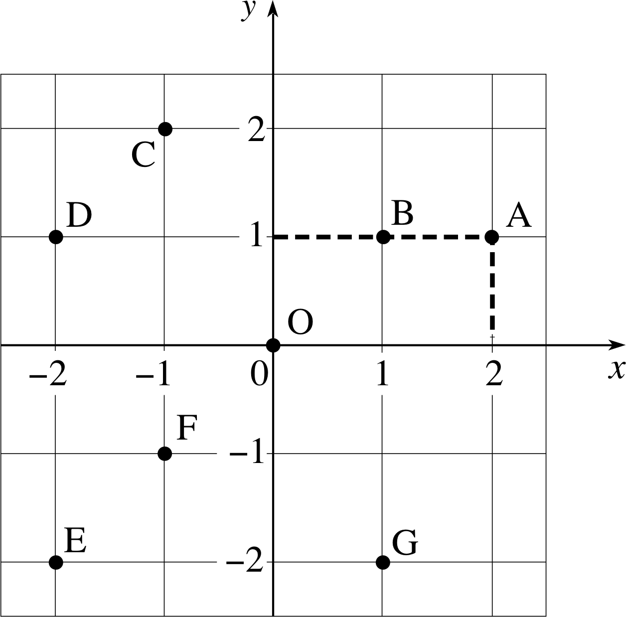
Figure 1 A Cartesian coordinate system and some points.
The framework used for drawing pictures of functions is that provided by Cartesian coordinates. Its basic ingredient is a pair of lines, called coordinate axes, at right angles to each other, as shown in Figure 1. The two lines may be regarded as infinitely long, extending as far as we like beyond the edges of the paper. By convention, the horizontal line is called the x–axis, and the vertical line the y–axis; the two lines intersect at a point called the origin. The lines are scaled to indicate the displacement from the origin. For the x–axis, displacements to the right of the origin are positive, and those to the left are negative; for the y–axis displacements above the origin are positive, and those below are negative. It is common to draw an arrowhead at the end of each axis to show the direction of increasing x or y.
Any pair of values for x and y can be represented by a point in the coordinate system. The pair (a, b) is represented by the point that is at a displacement a from the origin, measured parallel to the x–axis and a displacement b from the origin, measured parallel to the y–axis. i The point corresponding to the pair (2, 1) is shown as the point A in Figure 1; a perpendicular line from A to the x–axis meets it at x = 2, and a perpendicular line from A to the y–axis meets it at y = 1. Similarly the number pairs (1, 1) and (−1, 2), represent, respectively, the points B and C in Figure 1.
Question T4
What values of (x, y) represent the points D, E, F, G and O in E Figure 1?
Answer T4
D is (−2, 1), E is (−2, −2), F is (−1, −1), G is (1, −2) and O is (0, 0).
| x | f (x) = 2x + 1 |
|---|---|
| −2.0 | −3.0 |
| −1.5 | −2.0 |
| −1.0 | −1.0 |
| −0.5 | 0.0 |
| 0.0 | 1.0 |
| 0.5 | 2.0 |
| 1.0 | 3.0 |
| 1.5 | 4.0 |
| 2.0 | 5.0 |
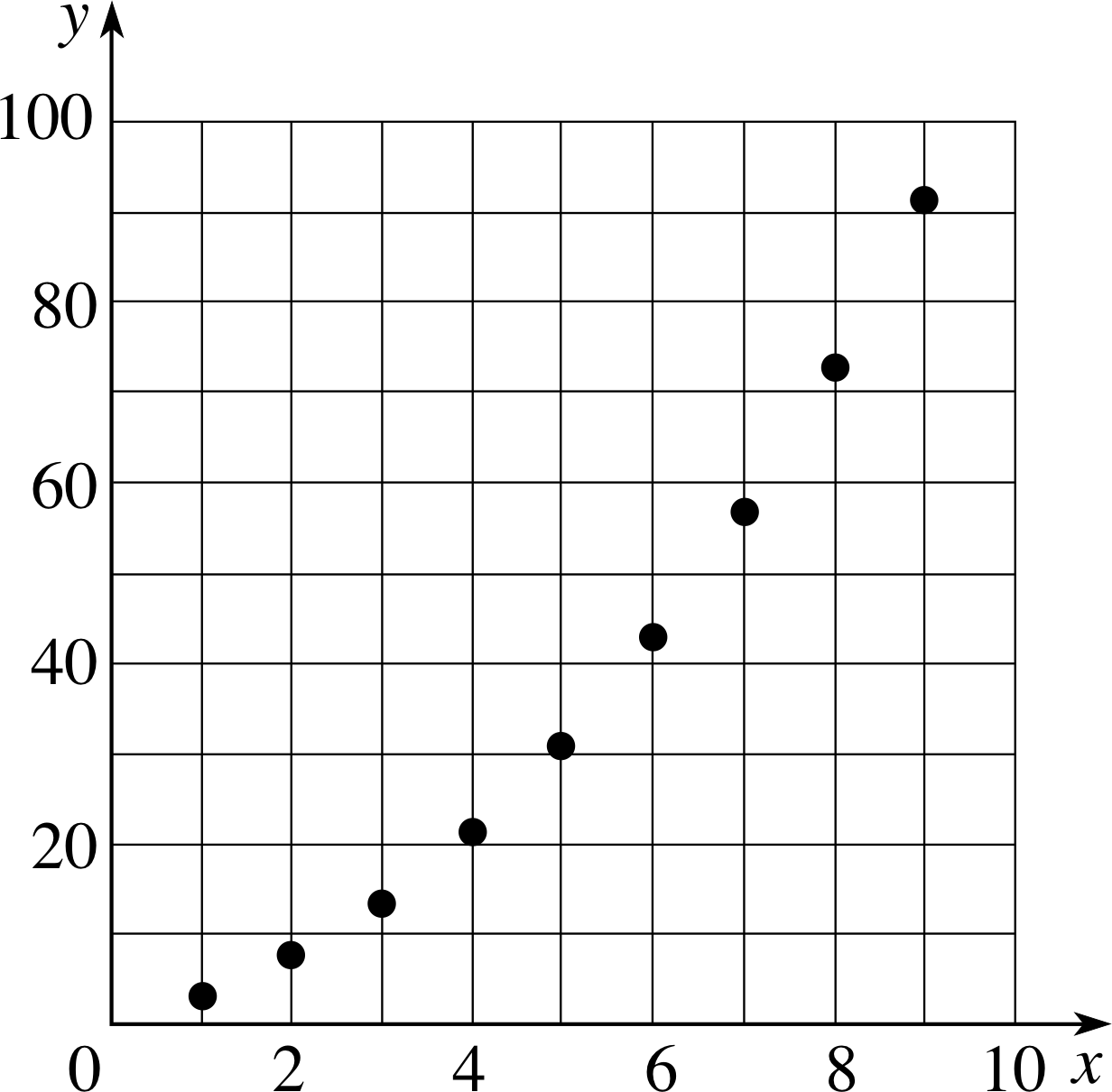
Figure 2 The graph of the function defined by Table 1.
3.2 Representing functions by graphs
Undoubtedly you will be familiar with the use of graphs to plot data; scientists use them all the time, and so do newspapers, but the idea of the graph of a function may be less familiar. Nonetheless, given a function f (x), any allowed value of x together with the corresponding function value y = f (x) forms a pair of numbers (x, y) that can be represented by a point in a Cartesian coordinate system. Figure 2 shows the result of plotting all such points for the function defined by Table 1. This plot is called the graph of the function. i
In science we are more often interested in continuous variables. If x is a continuous variable then there will be an infinite number of points (x, f (x)) which can be plotted on the diagram. Consider, for instance, the function
f (x) = 2x + 1(2) i
and let y = f (x). For every value of x we have a corresponding value of y. For x = 0, y = 1; for x = 1, y = 3; for x = −1, y = −1 and so on; these pairs of numbers can be used to compile a representative table of values (Table 2) that can be used to help us plot the graph of the function f (x).
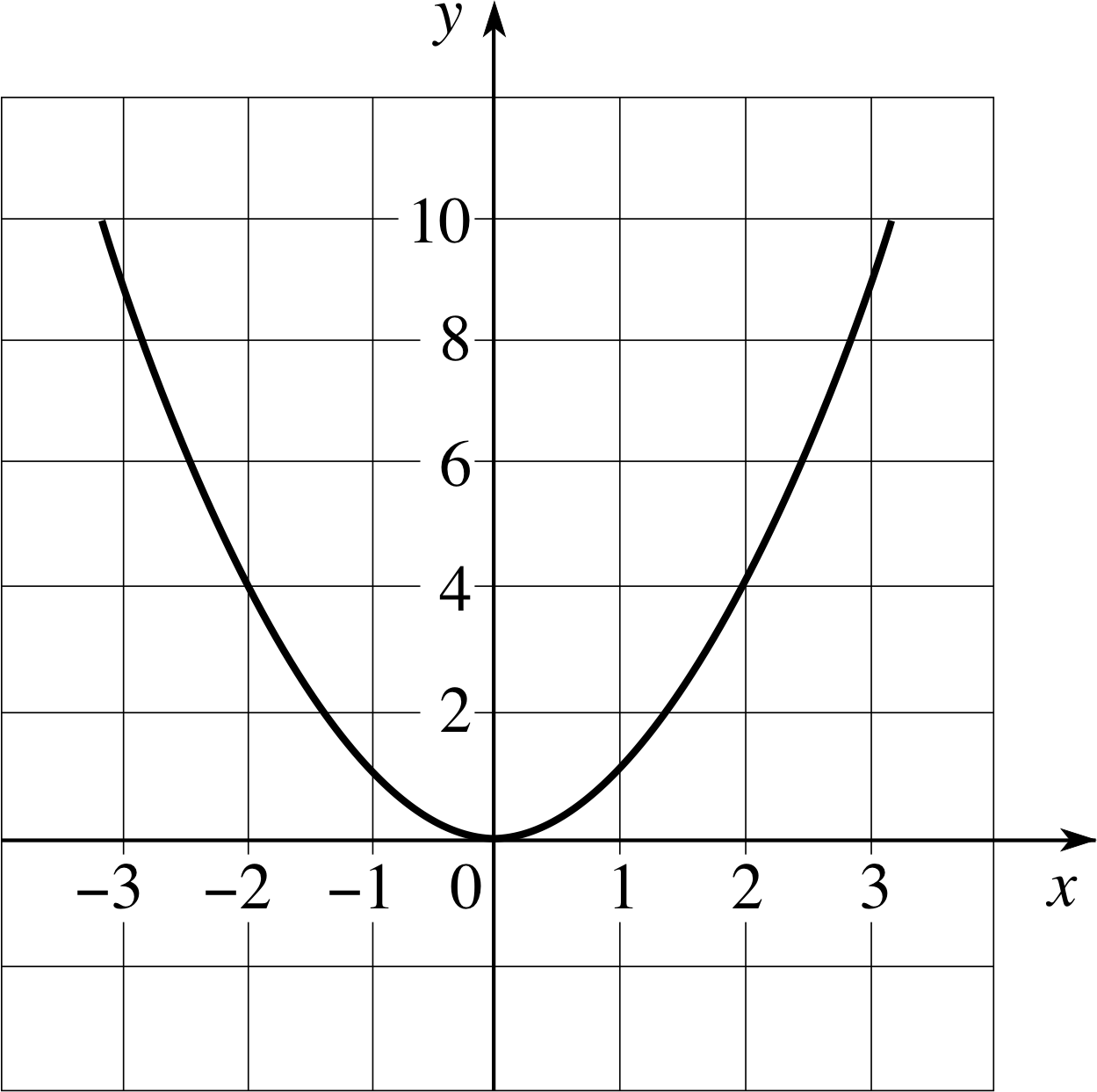
Figure 4 Graph of the function g (x) = x2.
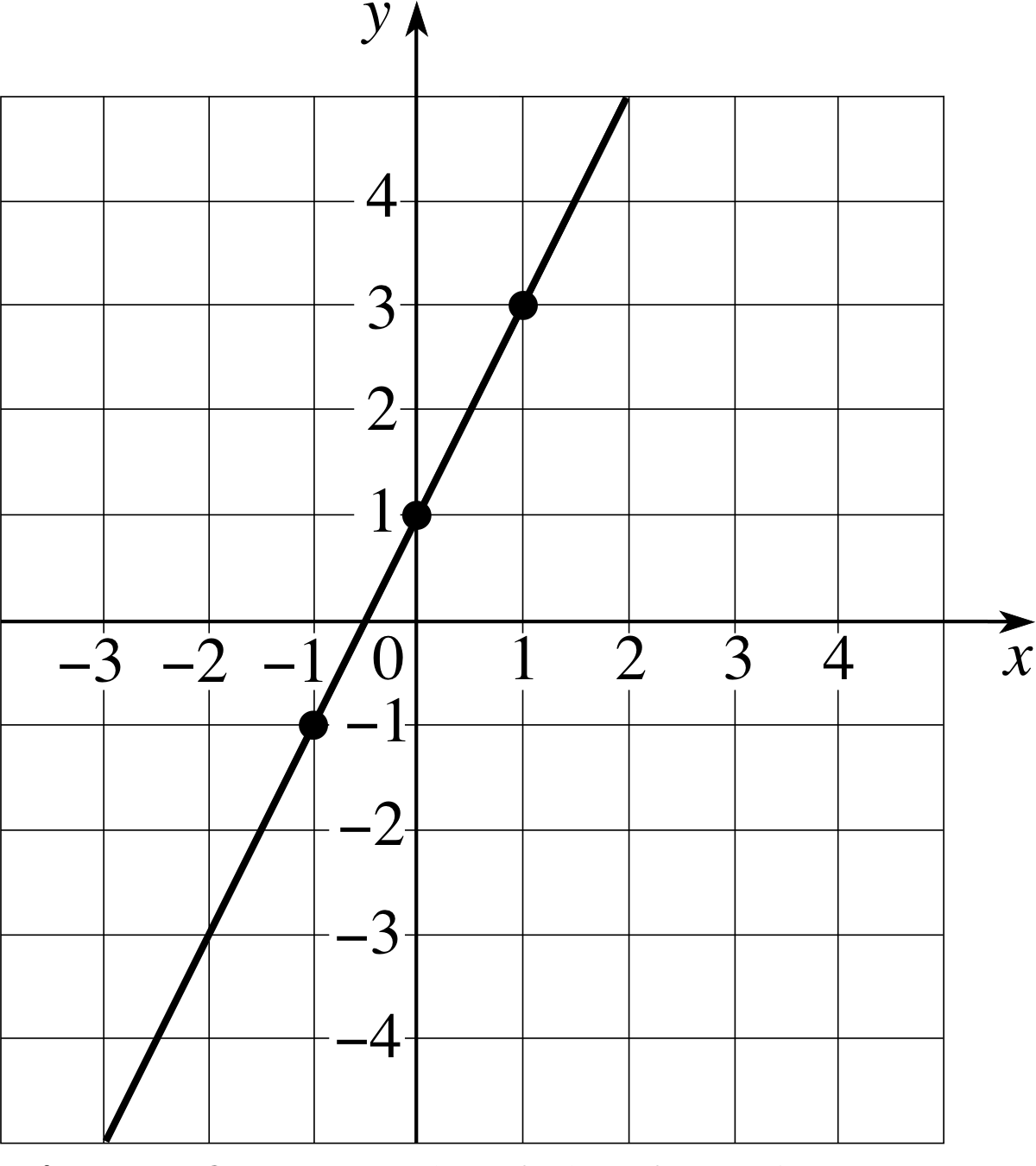
Figure 3 Graph of the function f (x) = 2x + 1.
After plotting just a few points it soon becomes clear that all the points lie on a straight line as shown in Figure 3.
Similarly the function
g (x) = x2(3)
will give the curve shown in Figure 4. Here again we have taken y = g (x); this is the customary way of proceeding, and in future we shall draw the graph of any function with an axis labelled as the y–axis.
From this we can see that any function may be characterized by its graph, and that a graph can show very simply many of the important behavioural features of a function. It is, of course, for this reason that graphs are so commonly used both inside and outside science.
3.3 Drawing and sketching graphs
A graph should convey a visual message, either to you personally, or (more importantly) to anyone else who may look at it. i You should therefore make sure that the information it presents is as clear and comprehensible as possible, just as you should do when writing something. Here are some points to pay attention to when drawing a graph.
Using graph paper Graph paper is necessary if any degree of accuracy is to be maintained, but it may not be needed for a quick sketch. The grid provided by the paper will limit your choice of scale and hence the size of the graph. You should not try to use the paper completely at the expense of a sensible scale. A 1 cm square, for example, may conveniently represent an interval of 1, 2, or 5 scale units, but 4 and certainly 3 should be avoided. A single experience of reading intermediate points from such a scale should convince you of this.
Selecting the size, scale and orientation The most important thing to do is to choose the right scales for both the horizontal and vertical axes. These should cover the whole range of interest, and a little more. The curves or points on the graph will then cover the whole area, with no unnecessary large blank areas at any of the edges. i
You can orientate your paper whichever way you want, but it is conventional to assign the horizontal axis to the independent variable and the vertical axis to the dependent variable.
Marking and numbering the axes Each axis should have the scale units indicated at reasonable intervals by graduation marks (small lines at right angles to the axis). There shouldn’t be too many of these marks, but enough so that the viewer can estimate the location of intermediate points without difficulty. Similarly, the numbers written along the axes to show the scale values associated with some of the graduation marks should not be too frequent – though you will usually need at least one number for every five graduation marks. Take care to choose sensible sequences of numbers; choices such as 1, 2, 3, ..., or 10, 20, 30, ..., are obvious, but if the whole range is large you might prefer to use 2, 4, 6, ..., or 5, 10, 15, ... . Avoid using sequences like 3, 6, 9, ...; even intervals of 4 may be found irritating. In brief, only display useful numbers, and try to avoid any appearance of ‘fussiness’ on the page.
Labelling the axes Points that physicists need to pay particular attention to when drawing graphs are labelling axes and indicating any units that have been used in the measurement of physical quantities. If you are plotting a purely numerical variable (without physical units) you have nothing to worry about, just put the name of the variable or the symbol representing it, (x or y or whatever) along the appropriate axis. However, if you are plotting values of variables such as mass or length that do require units it is usually best to label the axis as ‘mass/kg’ or ‘length/m’, as though dividing the variable by the relevant unit, it is then logical to write pure numbers along the axes rather than values that include units. i
If plotting very large or very small values it is generally a good idea to use multiples of units. For instance, if you have to plot masses in the range 2 × 10⁶ kg to 2 × 10⁷ kg it is probably best to label the axis ‘mass/106 kg’, so that the numbers are only in the range 2 to 20.
Joining the dots When drawing a graph, you will only be able to plot a finite number of points through which the curve must pass, and you will then have to think about the best way of joining them up. As a general rule, the points should be joined with a pencil line in the smoothest manner possible, and there should be no kinks or discontinuities unless there are good mathematical or physical reasons for them. Knowing when to expect such kinks or discontinuities is a skill that comes with insight and experience; this module is only the starting point for the development of such a skill.
The figures in this module should give you an idea of how to set out a graph in the proper way. i
So far we have talked about how to construct an accurate graph. This is usually called plotting_graphsplotting the graph. However, very often this plot is not necessary. If you are asked to sketching_graphssketch the behaviour of a function, rather than to draw or plot it, all that is needed is a rough diagram showing the main features. It should always be possible to deduce some of the following from the defining equation of the function:
- How does the function behave as x becomes large and positive?
- How does the function behave as x becomes large and negative?
- What is the value at x = 0 (i.e. where does it cross the y–axis)?
These characteristics are unlikely to be enough, and you will probably have to compute one or two more points; but on the whole you should try to do as few calculations as possible.
Try to make use of the general characteristics of the particular type of function you are sketching; some of these are described in the following subsections, others are discussed elsewhere in FLAP – particularly in the modules devoted to differentiation.
Question T5
Draw a graph showing the cost of posting a first class letter as a function of its mass. (In August 1993 the rates were: up to 60 g, 24 p; 60 g to 100 g, 36 p; 100 g to 150 g, 45 p; 150 g to 200 g, 54 p.)
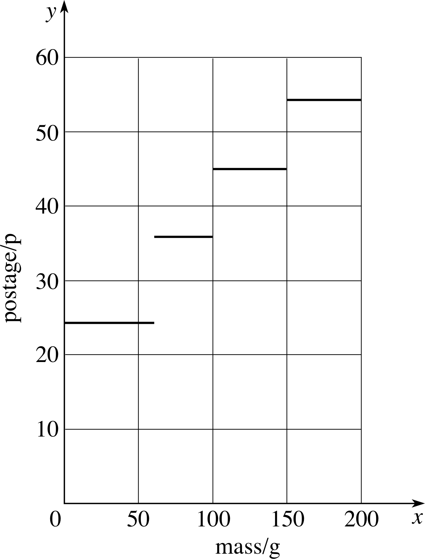
Figure 15 See Answer T5.
Answer T5
See Figure 15.
There are real discontinuities where the rate changes, so you should not try to join the lines up.
Question T6
Plot the graph of the function f (x) = x2 + x + 1 for x ≥ 0.
[Hint: remember the relationship between this function and the values in Table 1 or Figure 2.]
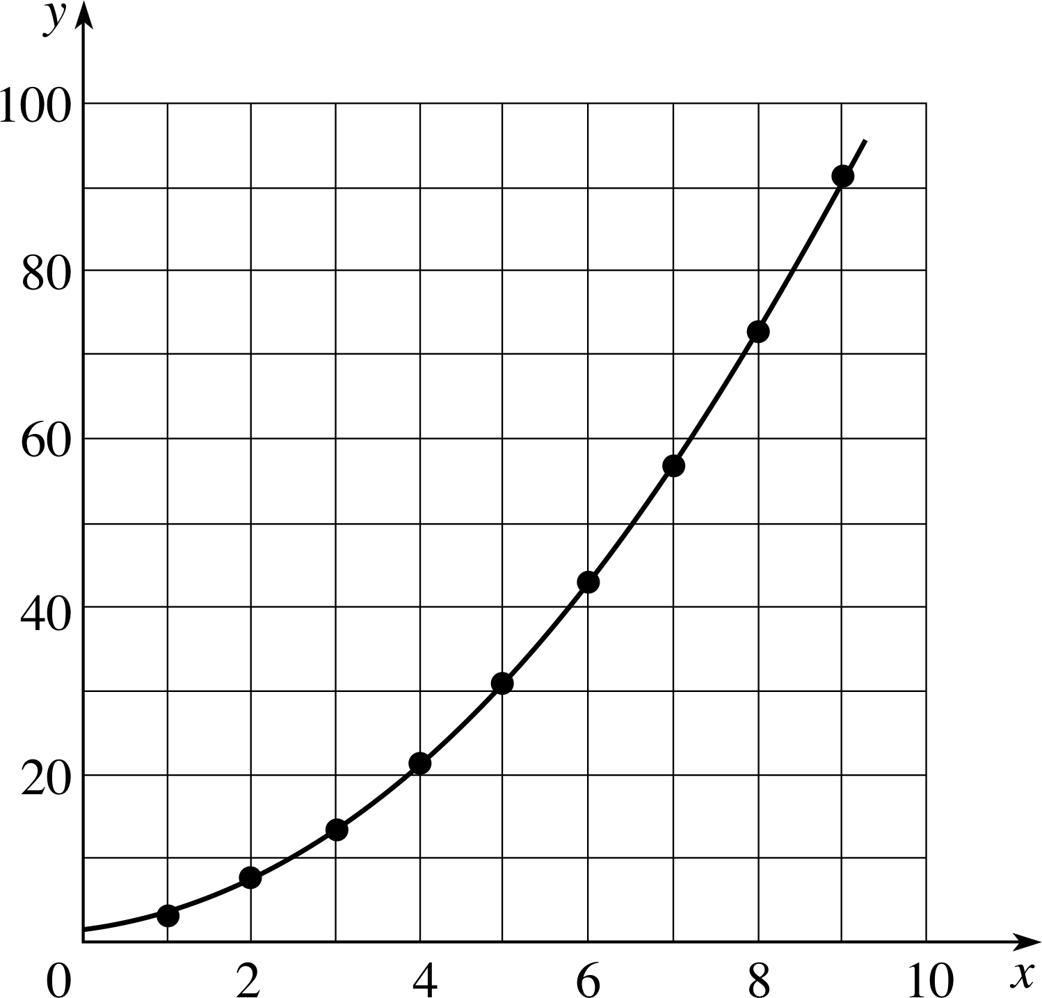
Figure 16 See Answer T6.
Answer T6
See Figure 16.
Draw the curve ‘with a flowing hand’. (It does not pass through the origin.)
The points supplied by Table 1 have been plotted as a guide to the curve.
3.4 Linear functions and straight–line graphs
In Subsection 3.2 you saw that the graph of the function f (x) = 2x + 1 was a straight line (Figure 3). Of course, this isn’t the only function to have a graph that is a straight line. In fact, there is an entire class of functions, called linear functions, every member of which has a straight–line graph.
A linear function is any function that may be written in the form
f (x) = mx + c(4)
where m and c are constants, called the gradient and intercept, respectively.
✦ Which of the following are linear functions? Give the values of the gradient m i and intercept c for each of the following linear functions.
(a) f (x) = 1 + 2x
(b) f (t) = −6.0 t − 3.8 × 10⁴
(c) f (x) = 6 x + a where a is a constant
(d) f (x) = cx + b where c and b are constants
(e) f (x) = 3x2 − 2.1
(f) f (x2) = 3x2 − 2.1 (Pay attention to the argument of this function)
✧ (a) f (x) is linear, it is equal to 2x + 1; m = 2, c = 1
(b) f (t) is linear; m = −6.0, c = − 3.8 × 10⁴
(c) f (x) is linear; m = 6, c = a (You may not know the value of a, but that makes no difference as long as you know it’s constant.)
(d) f (x) is linear; in this case the gradient is c and the intercept is b. Don’t be confused by the fact that the given function includes a constant called c. That constant has no connection whatsoever with the symbol c that is conventionally used to represent the intercept.
(e) f (x) is not linear, so the terms gradient and intercept do not apply.
(f) f (x2) is linear, but note that it is a linear function of x2 (though not a linear function of x). In other words if we let y = f (x2) and plot the graph of y against x2 the result will be a straight line (though a graph of y against x would not be straight). Regarded as a function of x2, the gradient is m = 3 and the intercept c = −2.1. i
The two constants that characterize any linear function are called the gradient and intercept for good reasons. To appreciate these reasons look again at Figure 3 – the graph of y = 2x + 1. Note that the straight line crosses the y–axis at y = 1, the value of the intercept. Also note that along the straight line the value of y increases twice as fast as the value of x, this factor of 2 corresponds to the gradient of the function which therefore determines the steepness or inclination of the graph.
These graphical interpretations of m and c are general properties, as we now show.
Figure 3 Graph of the function f (x) = 2x + 1.
Given any linear function f (x) the equation y = f (x) will describe a straight line. Thus, we may define
the general equation of a straight line
y = mx + c(5)
where m and c are constants.
In this general case, shown graphically in Figure 5a, any point on the y–axis is at x = 0, and substituting this value of x into Equation 5 shows that the general straight line intersects the y–axis at y = c.
Similarly, if x is increased by h (from x1 to x2 = x1 + h, say) then Equation 5 shows that y increases by mh from y1 = mx1 + c to y2 = m (x1 + h) + c = y1 + mh
so$\dfrac{y_2 - y_1}{x_2 - x_1} = \dfrac{mh}{h} = m$
This expression relating m to a change in y and to the corresponding change in x is very important. The symbols ∆x and ∆y, sometimes called the run and the rise, are used to represent the changes in x and y, so the gradient can be written in any of the following ways:
$\text{gradient} = \dfrac{\text{rise}}{\text{run}} = \dfrac{\text{change in }y}{\text{change in }x} = \dfrac{y_2-y_1}{x_2-x_1} = \dfrac{\Delta y}{\Delta x} = m$(6) i
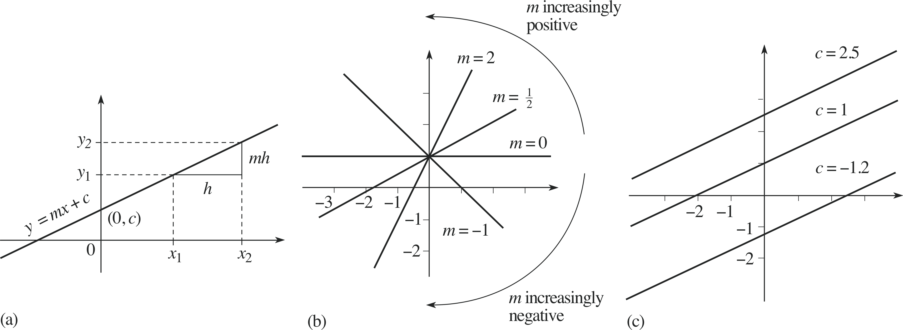
Figure 5 (a) The gradient–intercept form of a straight line, characterized by the constants m and c. (b) Changing the gradient m alters the steepness of the line. (c) Changing the intercept c alters the value of y at x = 0.
Figures 5b and 5c show, respectively, the effect on the graph of different values of m and c. Note that if m is zero the graph is horizontal whereas if m is negative the graph slopes downwards from left to right. The larger the value of m the ‘steeper’ the incline. Also note that if c is negative the intercept with the y–axis is below the x–axis.
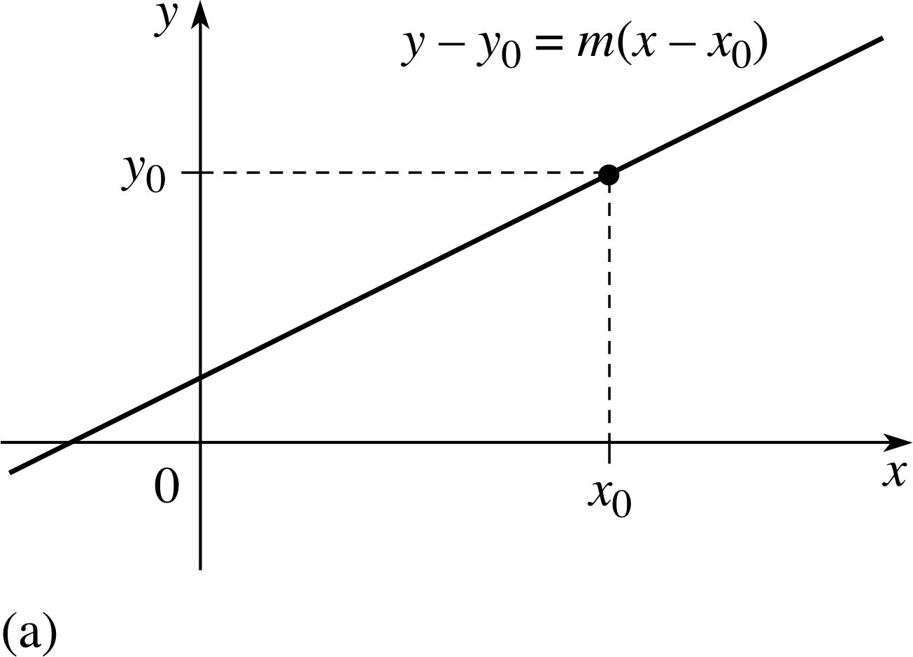
Figure 6a The point–gradient form of a straight line.
✦ Given a straight–line graph, how would you determine (a) the gradient, and (b) intercept of the corresponding linear function?
✧ (a) To find the gradient:
1 Pick two convenient points, (x1, y1) and (x2, y2), on the straight line.
2 Determine their horizontal separation x2 − x1. (This corresponds to the separation h in Figure 5a, and is often called the run.) i
3 Determine their vertical separation y2 − y1, taking the points in the same order as before. (This corresponds to the separation mh in Figure 5a and is often called the rise.)
4 Then, from Equation 6,
${\rm gradient} = \dfrac{\rm rise}{\rm run} = \dfrac{y_2-y_1}{x_2-x_1}$
(b) To find the intercept:
Simply find the value of y that corresponds to x = 0. (Note if your graph does not include x = 0, do not make the mistake of taking the value of y at which the line crosses your vertical axis to be the intercept. It must be the y value at x = 0).
The gradient–intercept form (Equation 5) is one of the commonest ways of representing the equation of a straight line or the corresponding linear function, but there are other representations which are also useful. For example, if we know the gradient m of a line and the fact that it passes through the point (x0, y0), then the equation of the line can be written
y − y0 = m (x − x0)(7)
this is called the point–gradient form and is illustrated in Figure 6a.
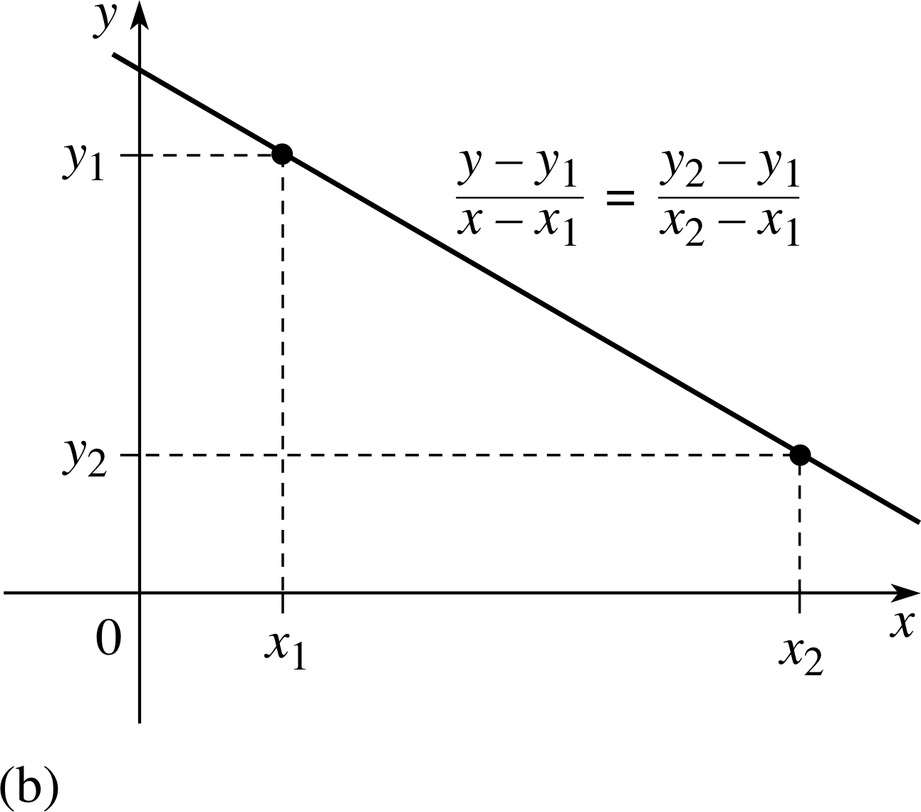
Figure 6b The two–point form of a straight line.
Question T7
Rearrange Equation 7 to show that it is equivalent to Equation 5,
y = mx + c(Eqn 5)
and find the value of the intercept implied by Equation 7.
Answer T7
y − y0 = m (x − x0), therefore y − y0 = mx − mx0
So, y = mx − mx0 + y0, hence the gradient is m and the intercept y0 − mx0.
It is well known that given two points, (x1, y1) and (x2, y2) there is a unique straight line joining them; in other words two points determine a straight line. This fact provides the basis of another way of writing the equation of a straight line – the two–point form (illustrated in Figure 6b)
$\dfrac{y-y_1}{x-x_1} = \dfrac{y_2-y_1}{x_2-x_1}$(8)
Question T8
Rearrange Equation 8 to show that it is also equivalent to Equation 5 and again find the implied value of the intercept.
Answer T8
First of all note that, from Equation 6, the right–hand side of Equation 8 is just equal to m. So we can write Equation 8 as (y − y1)/(x − x1) = m.
If this is then rearranged, y − y1 = m (x − x1), which is in the same form as Equation 7.
Therefore the answer follows from Answer T7, the intercept is y1 − mx1.
Yet another standard form for the equation of the straight line is
$\dfrac xa + \dfrac yb = 1$(9)
This is known as the intercept form.
Question T9
What is the graphical significance of the constants a and b in Equation 9?
Answer T9
When x = 0, y/b = 1, so y = b. When y = 0, x/a = 1, so x = a.
Hence a and b are the intercepts where the straight line cuts the x– and y–axes, respectively.
3.5 Quadratic functions and turning points
Linear functions and straight–line graphs are very common in mathematics and physics, but there are many other functions which are also important. The quadratic function, a function of x which contains no higher power of x than x2 is one such function.
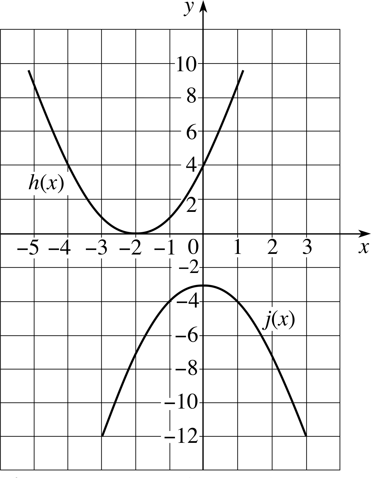
Figure 7 Graphs of the quadratic functions h (x) = (x + 2)2 and j (x) = −x2 − 3
A quadratic function is any function that may be written in the form
f (x) = ax2 + bx + c(10)
where a, b and c are constants.
A simple example of a quadratic function was shown in Figure 4; it was the function
g (x) = x2(Eqn 3)
which is obtained by setting a = 1, b = 0 and c = 0 in Equation 10. Two other quadratic functions, corresponding to different choices of a, b and c are shown in Figure 7, they are
h (x) = (x + 2)2(11) i
andj (x) = −x2 − 3(12)
There are some important features that are common to all three of these examples of quadratic equations:
- For each function there is a turning point, i.e. a point at which the value of the function ceases to increase or decrease and the graph turns back on itself. For quadratic functions the turning point is either a minimum or a maximum value of the function. i
- For each function, the graph is symmetrical about a vertical line drawn through the turning point. The graphical curve defined by a quadratic function is called a parabola and the turning point is called the vertex_of_a_parabolavertex of the parabola.
✦ What are the values of a, b and c (as given in Equation 10) for the functions h (x) and j (x)?
✧ For h (x); a = 1, b = 4, c = 4
For j (x); a = −1, b = 0, c = −3
For any quadratic function, the values of the constants a, b and c determine the precise shape and location of the corresponding parabola.
For instance, if a is positive the vertex is at the ‘bottom’ of the parabola and thus represents the minimum value of y. If a is negative, the vertex is at the ‘top’ of the parabola and corresponds to a maximum value of y. Moreover, the precise value of a determines the ‘width’ of the parabola. The function
$k(x) = \left(\dfrac x2\right)^2$(13)
is twice as ‘wide’ as the function g (x) = x2 for a given value of x.
Question T10
Sketch the graphs of k (x) and g (x) (Equations 13 and 3, respectively) and thus confirm the claim made above about the role of a in determining the ‘width’ of the parabola.
$g(x) = x^2$(Eqn 3)
$k(x) = \left(\dfrac x2\right)^2$(Eqn 13)
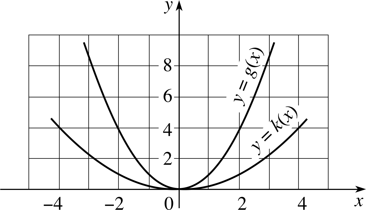
Figure 17 See Answer T17.
Answer T10
The graphs of k (x) and g (x) are sketched in Figure 17.
The constants a, b and c also determine the location of the parabola’s vertex.
Inspecting the graphs of Figure 7, you should be able to convince yourself that:
- the vertex of h (x) = (x + 2)2 is at the point (−2, 0)
- the vertex of j (x) = −x2 − 3 is at the point (0, −3).
These are two special cases of a more general result, namely that the vertex of any quadratic function of the form a (x − p)2 is at (p, 0) and the vertex of any quadratic function of the form ax2 + q is at (0, q).
Question T11
(a) Write down a general expression for a quadratic function with a vertex at the point (p, q).
(b) Write down the quadratic functions with a = 1 which have vertices at the points (i) (1, 3) (ii) (−2, 1) and (iii) (2, −1). Sketch the graphs of these functions. i
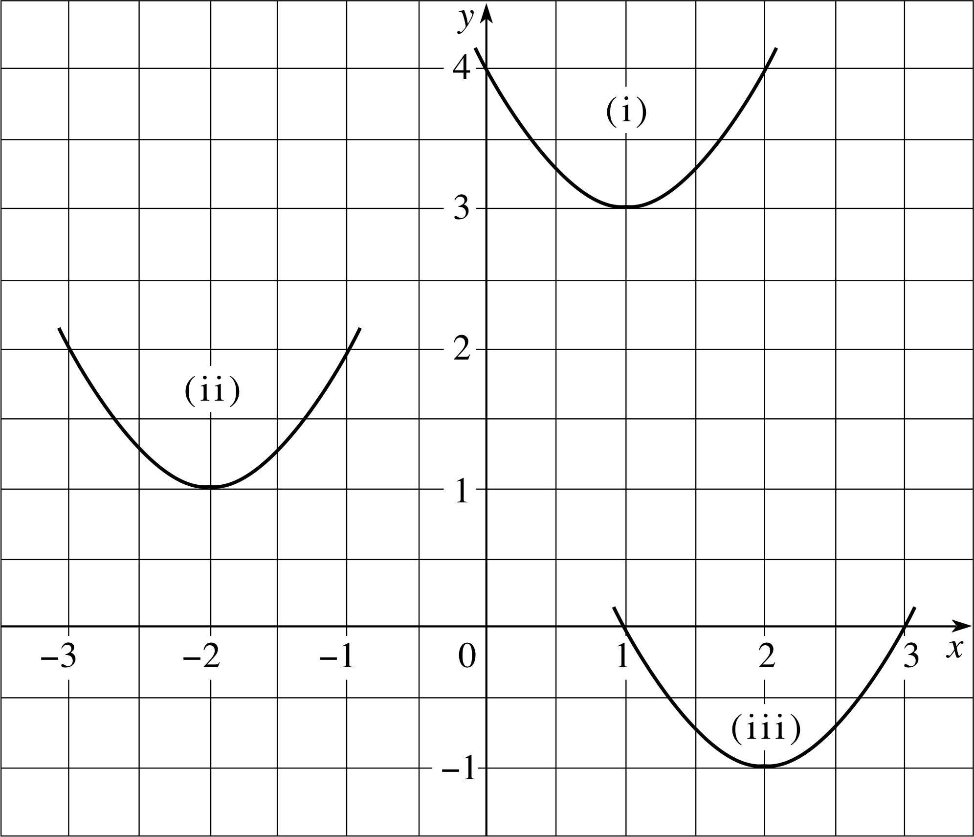
Figure 18 See Answer T18(b).
Answer T11
(a) As you know the vertex of a (x − p)2 is at (p, 0) you should be able to see that the required quadratic function has the form
f (x) = a (x − p)2 + q
since the additional q will have the effect of moving each point on the parabola, including the vertex, q units upwards.
(b) The quadratic functions (and vertices) are:
(i) f (x) = (x − 1)2 + 3 vertex at (1, 3)
(ii) f (x) = (x + 2)2 + 1 vertex at (−2, 1)
(iii) f (x) = (x − 2)2 − 1 vertex at (2, −1)
They are sketched in Figure 18. Note that each has the same ‘width’ since a is the same in each case.
Given any quadratic function f (x), or the equation of the corresponding parabola y = f (x), the items of information most often of interest are the position of the vertex and the locations of any points at which the parabola intersects the x and y axes. The position of the vertex can always be found by a process known as completing the square, the intersections (if they exist) can be found by factorization. We will deal with these processes in turn.
The completed square form of a quadratic function is:
f (x) = a (x − p)2 + q(14)
where a, p and q are constant.
As indicated in the answer to Question T11, the graph of this function has its vertex located at the point (p, q).
The process of completing the square allows us to rewrite any given quadratic f (x) = ax2 + bx + c in the completed square form of Equation 14. To see that this is possible just note that
$ax^2+bx+c = a\left(x^2+\dfrac{b}{a}x+\dfrac{c}{a}\right) = a\left[\left(x+\dfrac{b}{2a}\right)^2-\dfrac{b^2}{4a^2}+\dfrac{c}{a}\right]$ i
and thus$ax^2+bx+c = a\left(x+\dfrac{b}{2a}\right)^2-\dfrac{b^2}{4a}+c$(15)
We have now managed to isolate x within the brackets, just as in the completed square form (Equation 14). Comparing Equations 14 and 15 you should be able to see that they are the same if we make the following identifications
$p = \dfrac{-b}{2a} \quad\text{and}\quad q = \dfrac{-b^2}{4a}+c$
Thus, the vertex of the parabola y = ax2 + bx + c is located at the point
$\left(\dfrac{-b}{2a},\,\dfrac{-b^2}{4a}+c\right)$
We now turn to the problem of determining the points at which the parabola y = ax2 + bx + c intersects the x and y–axes.
The intersection with the y–axis occurs when x = 0, so it follows from the equation of the parabola that at the point of intersection, y = c.
The parabola does not necessarily intersect the x–axis at all – the graph of j (x) in Figure 7 has no such intersection, though h (x) meets, rather than intersects, the axis once and one of the parabolas you drew in answering Question T11 has two such intersections. However, if the graph of f (x) = ax2 + bx + c does cross the x–axis at two points, let’s say at x = α and x = β, then it is always possible to find those points by writing the quadratic in the so called factorized form:
f (x) = a (x − α)(x − β)(16)
where a, α and β are constant.
Expanding this expression certainly gives a quadratic, since
f (x) = a [x2 − (α + β)x + αβ]
Moreover, if we substitute x = α into Equation 16 you can see that f (α) = 0 and similarly if x = β, f (β) = 0.
So the graph of this particular quadratic does indeed intersect the x–axis at x = α and x = β.
A general quadratic may always be written in the factorized form of Equation 16. The process by which the factorized form of a quadratic is determined is called factorization. Sometimes, in very simple cases, it is possible to deduce the factorized form simply by ‘inspecting’ the original quadratic (this becomes easier with experience). More generally, it is always possible to use the following formula to find the values of x at which points of intersection occur, and hence the values of α and β.
If the parabola y = ax2 + bx + c intersects the x–axis, it does so at the points
$x = \dfrac{-b\pm\sqrt{b^2-4ac}}{2a}$(17)
The symbol ± is read as ‘plus or minus’ and reminds us that this single equation generally provides two values for x. i
It is worth noting that this formula provides the values of α and β in the factorized form of a quadratic (Equation 16) even when α and β do not correspond to distinct points of intersection with the x–axis. The quantity b2 − 4ac that appears under the square root symbol in Equation 17 is called the discriminant and it is this that determines the number of times the graph of the quadratic function ax2 + bx + c meets or crosses (intersects) the x–axis.
- If b2 − 4ac > 0, there will be two crossing points with x–coordinates given by Equation 17.
- If b2 − 4ac = 0, there is only a single meeting point at x = −b/(2a).
- If b2 − 4ac < 0, there is no real number equal to b2 − 4ac and the parabola will not meet or cross the x–axis at all.
It is also worth noting that, since y = 0 when the parabola intersects the x–axis, the two values of x given by Equation 17 must satisfy an equation of the following form. i
ax2 + bx + c = 0(18)
Equations of this kind are called quadratic equations, they are common in Physics and are dealt with in more detail elsewhere in FLAP.
Question T12
For each of the following quadratic functions, determine the number of times its graph meets or crosses the horizontal axis, rewrite the function in completed square form and thus determine the location of the vertex:
(a) f (x) = 3x2 − 9x + 11 (b) f (t) = −t2 − 2t − 6 (c) f (R) = −3R2 + 15R − 18
Answer T12
(a) f (x) = 3x2 − 9x + 11 does not intersect the x–axis since its discriminant is negative. In completed square form (see Equation 14)
$f(x) = 3\left(x-\dfrac32\right)^2 +\dfrac{17}{4}$
So its vertex (a minimum) is at (3/2, 17/4).
(b) f (t) = −t2 − 2t − 6 does not intersect the t–axis since its discriminant is negative. In completed square form
f (t) = −(t + 1)2 − 5
so its vertex (a maximum) is at (−1, −5)
(c) f (R) = −3R2 + 15R − 18 intersects the R–axis twice since its discriminant is greater than zero. In completed square form
$f(R) = -3\left(R - \dfrac52\right)^2 + \dfrac34$
so its vertex (a maximum) is at (5/2, 3/4)
Question T13
For each of the following quadratic functions, determine the points (if there are any) at which its graph intersects the horizontal axis:
(a) f (y) = y2 + 5y − 1 (b) f (t) = 2t2 − 3t + 4 (c) $f(Z) = 3Z^2 + \dfrac Z2 - \dfrac14$ (d) f (x) = x2 − 5x + 6
Answer T13
(a) $y = \dfrac{-5 \pm \sqrt{25 + 4\os}}{2} = -5.193 \;\text{and}\; 0.193$
(b) The discriminant is less than zero, so there are no points of intersection.
(c) $Z = \dfrac{-0.5 \pm \sqrt{0.25 + 3\os}}{6} = 0.217 \;\text{and}\; -0.384$
(d) $x = \dfrac{5 \pm \sqrt{25 - 24\os}}{2} = 3 \;\text{and}\; 2$
In simple cases such as (d) it is not always necessary to use the formula to find the points of intersection. With practice you should be able to see ‘by inspection’ the factorized form of the function: x2 − 5x + 6 = (x − 2)(x − 3).
Practice at developing this skill is given elsewhere in FLAP.
3.6 Polynomial functions and points of inflection
Linear and quadratic functions are simple examples of a wider class of functions that may involve higher powers of a variable.
A polynomial function of degree_of_a_polynomialdegree n is any function of the form
f (x) = a0 + a1x + a2x2 + ... + an−2 x n−2 + an−1x n−1 + anx n(19)
where n is an integer, and the n + 1 constants a0, a1, a2, ... an−2, an−1 and an are called the coefficients of the polynomial, with a n not equal to zero. i
Thus, a polynomial function of x of degree n involves powers of x up to and including x n but no higher powers. A linear function is a polynomial of degree 1, and a quadratic function is a polynomial of degree 2.
✦ Polynomial functions of degree 3 and degree 4 are called cubic functions and quartic functions, respectively. Write down general expressions for such functions similar to those given earlier for linear and quadratic functions, Equations 4 and 10, respectively.
✧ f (x) = a + bx + cx2 + dx3 is a cubic function.
f (x) = a + bx + cx2 + dx3 + ex4 is a quartic function. i
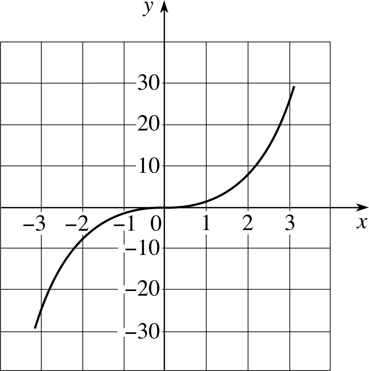
Figure 8 The cubic function f (x) = x3.
Such functions, not surprisingly, are much more complicated, and show more varied behaviour, than linear and quadratic ones. The simplest cubic function:
f (x) = x3(20)
has the graph shown in Figure 8. The two features to note about this are:
- 1
-
The behaviour of the graph far from the origin, where f (x) ≫ 0 for x ≫ 0, and f (x) ≪ 0 for x ≪ 0. i
- 2
-
The behaviour near the origin, where the graph changes from a downward turning curve for x < 0, to an upward turning curve for x > 0. This behaviour is typical of cubic functions and is often seen in other polynomials; the point at which the change of curvature occurs (the origin in this case) is called the point of inflection. i
Figure 9 The cubic function g (x) = x3 − 4x.
Other cubic functions with different coefficients can show more complicated behaviour. For example, consider the cubic function
g (x) = x3 − 4x(21)
The graph of this, shown in Figure 9, has the extra features of a (local) minimum near x = 1 and a (local) maximum near x = −1, in addition to the point of inflection at x = 0. i This is the greatest degree of complication which arises with cubic functions; different choices for the coefficients a, b, c and d would alter the detailed shape of the curve and the locations of the point of inflection and the turning points (if there are any), but no choice of coefficients results in more than one point of inflection and two turning points.
Clearly when dealing with higher degree polynomials the complications will become even worse, so we shall not pursue individual cases any further here.
The only general points to be noted are that for a polynomial function of degree n:
- There will be at most a total of (n − 1) local maxima and local minima.
- Between every local minimum and its neighbouring local maximum there will be a point of inflection.
- If n is even there will always be at least one maximum or minimum.
- If n (greater than 1) is odd there will always be at least one point of inflection.
3.7 Reciprocal functions and asymptotes
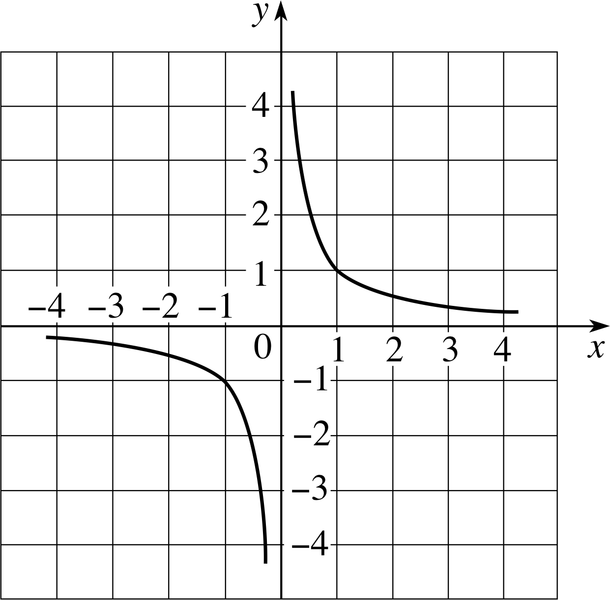
Figure 10 The hyperbola R (x) = 1/x.
Although polynomial functions are important, they are not the only kind of function you are likely to meet. Another very common function is the reciprocal function
R (x) = 1/x where x ≠ 0(22) i
the behaviour of which is shown in Figure 10. The shape of this curve is known as a hyperbola and shows a number of interesting features:
- The function R (x) is not defined for x = 0. So in this case the argument x may be any real number except 0.
- The curve consists of two separate pieces, one for x > 0, and one for x < 0.
- As x approaches zero, R (x) becomes large and positive if x > 0, but it becomes large and negative if x < 0.
The y–axis in Figure 10 forms a sort of limit which the curve approaches but never meets, no matter how far it is extended in either direction. Such a limiting line is called an asymptote, and the curve is said to approach it asymptotically. In this case the x–axis also forms an asymptote, since the curve never meets that either, though it approaches the asymptote more and more closely as x becomes increasingly positive or negative.
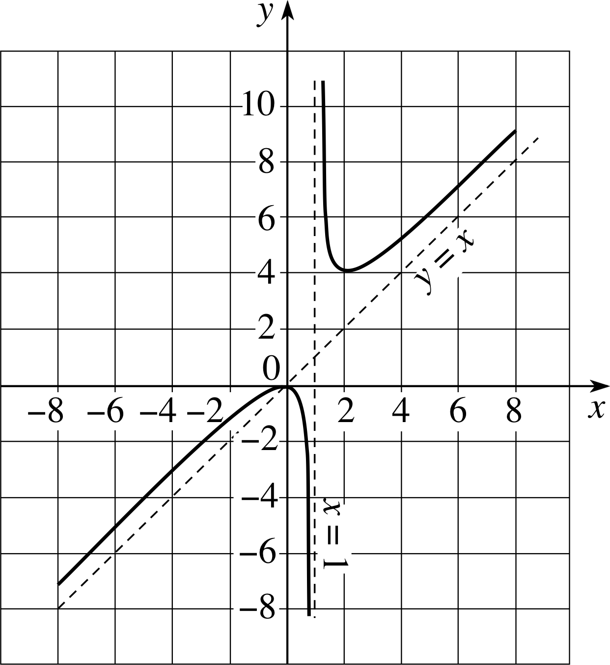
Figure 11 The graph of g (x) = x2/(x − 1) and its asymptotes.
Asymptotes do not have to be vertical or horizontal. Consider the function
g (x) = x2/(x − 1) where x ≠ 1(23)
and its graph in Figure 11. From what was said above it should be clear that x = 1 is a vertical asymptote. There is no horizontal asymptote in this case, but if we make x very large and positive, then the denominator (x − 1) is very nearly equal to x, so that g (x) ≈ x i, and the larger x becomes, the closer the curve comes to the line y = x, which is an asymptote.
We can use the same argument as x becomes large and negative.
When investigating the asymptotes of a function we are bound to be interested in some quantity (either x or y, usually) that is becoming either very large and positive or very large and negative. To aid such discussions it is useful to introduce the infinity symbol ∞ which is usually read as ‘infinity’. This symbol should not be thought of as a number; rather it represents a quantity that is much larger than any other quantity that is likely to be considered. When discussing asymptotes we can then discuss the behaviour as x or y approaches ∞ or −∞. For simplicity this is often written x → ∞ or x → − ∞. You should avoid writing x = ± ∞ since, as already stated, ∞ is not a number.
Question T14
(a) Sketch the curves and asymptotes for the function
f (x) = x/(x + 1) where x ≠ −1(24)
(b) What are the asymptotes of
g (x) = 2x2/(3x + 1)?
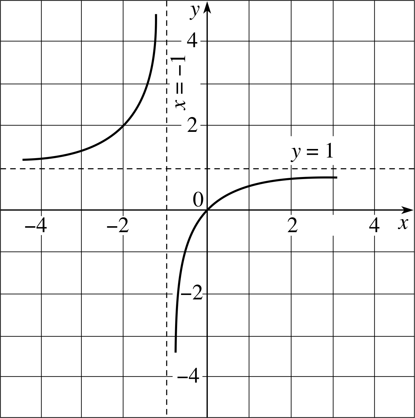
Figure 19 See Answer T14.
Answer T14
(a) See Figure 19. The asymptotes are the lines y = 1 and x = −1, i.e. as x → ± ∞, y → 0 and when x = −1 the denominator = 0.
(b) g (x) also has a vertical asymptote, at x = −1/3, but there is no horizontal asymptote. Instead, as x → ± ∞, g (x) ≈ 2x2/(3x) = 2x/3. So, the line y = 2x/3 is also an asymptote.
4 Inverse functions and functions of functions
4.1 Inverse functions
Figure 3 Graph of the function f (x) = 2x + 1.
The statement y = F (x) clearly indicates that y is a function of x, but sometimes it is very useful to look at things the other way round, and treat x as a function of y. As you will see shortly, it is not always possible to do this, but if it can be done the process will define a new function called the inverse function of F (x). Formally:
The inverse function of F (x) is a function G (y) such that if y = F (x), then x = G (y) for every value of x in the domain of F (x).
Loosely speaking the effect of the function F (x) is ‘undone’ by its inverse function G (y). i
Examples of inverse functions are easy to find. For instance in Subsection 3.2 we examined the function
f (x) = 2x + 1(Eqn 2)
the graph of which was shown in Figure 3. The inverse function of f (x) is
g (y) = ½ (y − 1)(25)
✦ Confirm the claim that g (y) (Equation 25) is the inverse of x f (x) (Equation 2) for the specific values x = −2, x = 0 and x = 3.
g (y) = 12 (y − 1)(Eqn 25)
f (x) = 2x + 1(Eqn 2)
✧ When x = −2, y = f (−2) = 2 (−2) + 1 = −3, and when y = −3, g (−3) = (−3 − 1)/2 = −2
When x = 0, y = f (0) = 2 (0) + 1 = 1, and when y = 1, g (1) = (1 − 1)/2 = 0
When x = 3, y = f (3) = 2 (3) + 1 = 7, and when y = 7, g (7) = (7 − 1)/2 = 3
So, for these three values of x at least, the functions f (x) and g (y) satisfy the requirement that g (y) should ‘undo’ the effect of f (x).
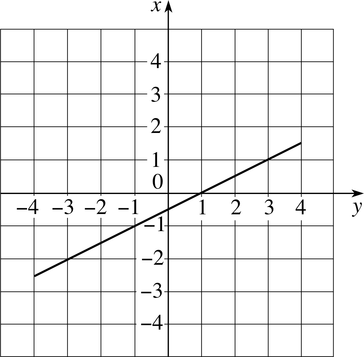
Figure 12 The graph of the function g (y) = (y − 1)/2, the inverse of the function f (x) = 2x + 1 shown in Figure 3. (Note the axes.)
The relationship between the functions f (x) and g (y) is perhaps more easily understood by noting that if
y = 2x + 1(26)
then x = ½ (y − 1)
So, in this particular case the form of the inverse function can be found by simply rearranging Equation 26. (Not all cases are so simple.)
More significantly, if you examine the graph of g (y), shown in Figure 12, and compare it with the graph of f (x), shown in Figure 3, you will see that the two graphs are related by a simple interchange of axes.
Although the inverse of f (x) has been called g (y) and its graph in Figure 12 has been plotted with y (the independent variable in this case) along the horizontal axis there is no need to show it in that way. Remember, given any function, its value is determined by the value of its argument – what you call the argument makes no difference.
Thus, given
g (y) = ½ (y − 1)(Eqn 25)
we can represent exactly the same function by
g (x) = ½ (x − 1)
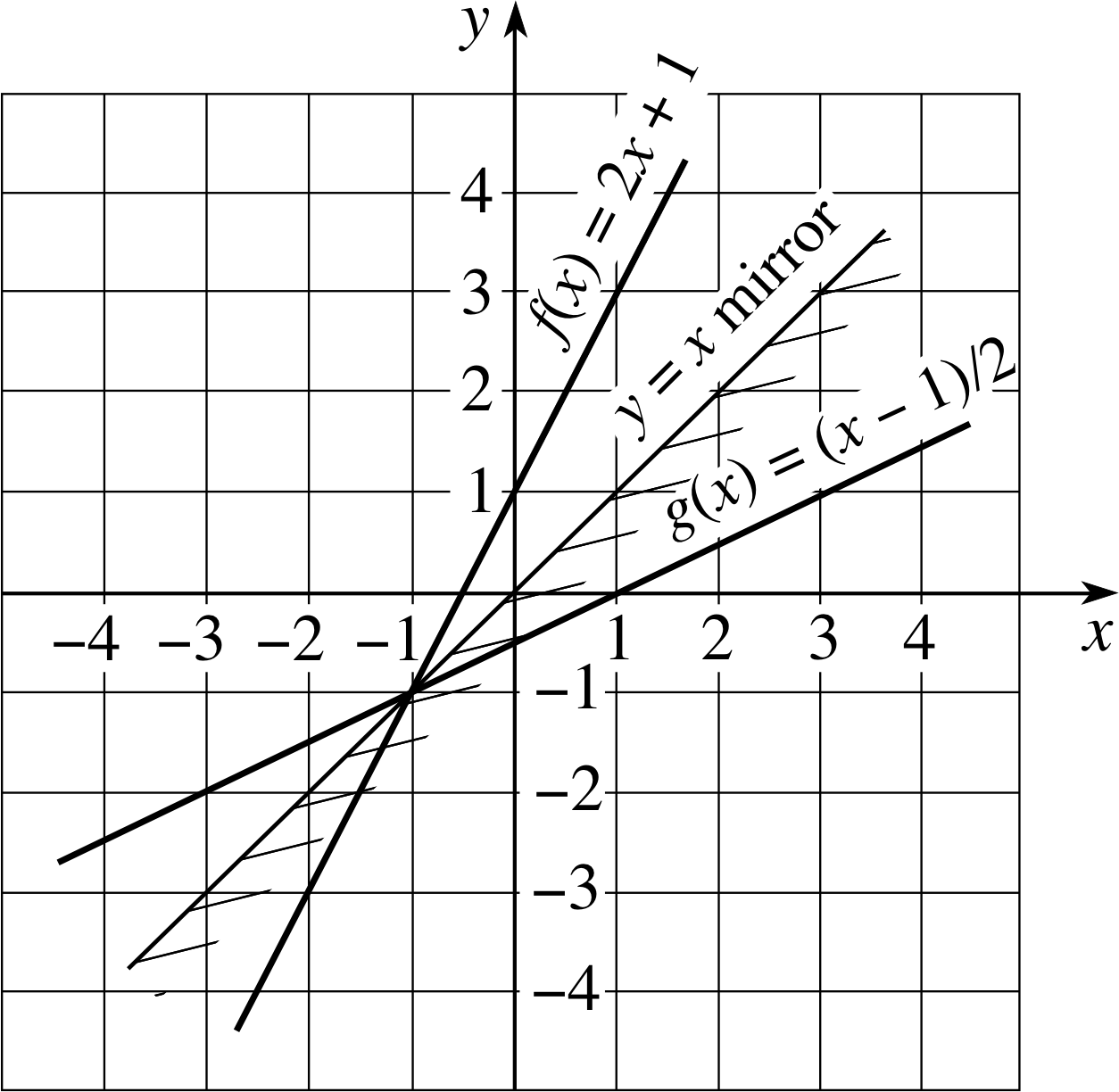
Figure 13 The function f (x) = 2x + 1 and its inverse g (x) = (x − 1)/2. These two lines are mirror images of each other in an imaginary mirror along the line y = x.
Thanks to this, there is no need to introduce unconventional axes, such as those in Figure 12, when drawing the graph of an inverse function. In fact, given a function f (x) and its inverse function g (x) we can plot both functions on the same axes. i
Doing so, as in Figure 13, reveals an interesting phenomenon – the line y = g (x) representing the inverse function can always be obtained by ‘reflecting’ the line y = f (x) in an imaginary mirror placed along the line y = x. (This imaginary mirror is also indicated in Figure 13). This ‘reflection symmetry’ between a function and its inverse is a general property, so given the graph of any function you can easily visualize the graph of its inverse – if that inverse exists. The proviso ‘if that inverse exists’ is an important one. Any graph may be ‘reflected’ but not every such reflection is the graph of an inverse function.
For example, the function g (x) = x2 (Eqn 3) was introduced in Subsection 3.2. (Do not confuse this function with the linear function g (x) that was considered above. This is a different example.) The graph of Equation 3 is the parabola that was plotted in Figure 4. The reflection of that graph in an imaginary mirror along the line y = x is shown in Figure 14a.
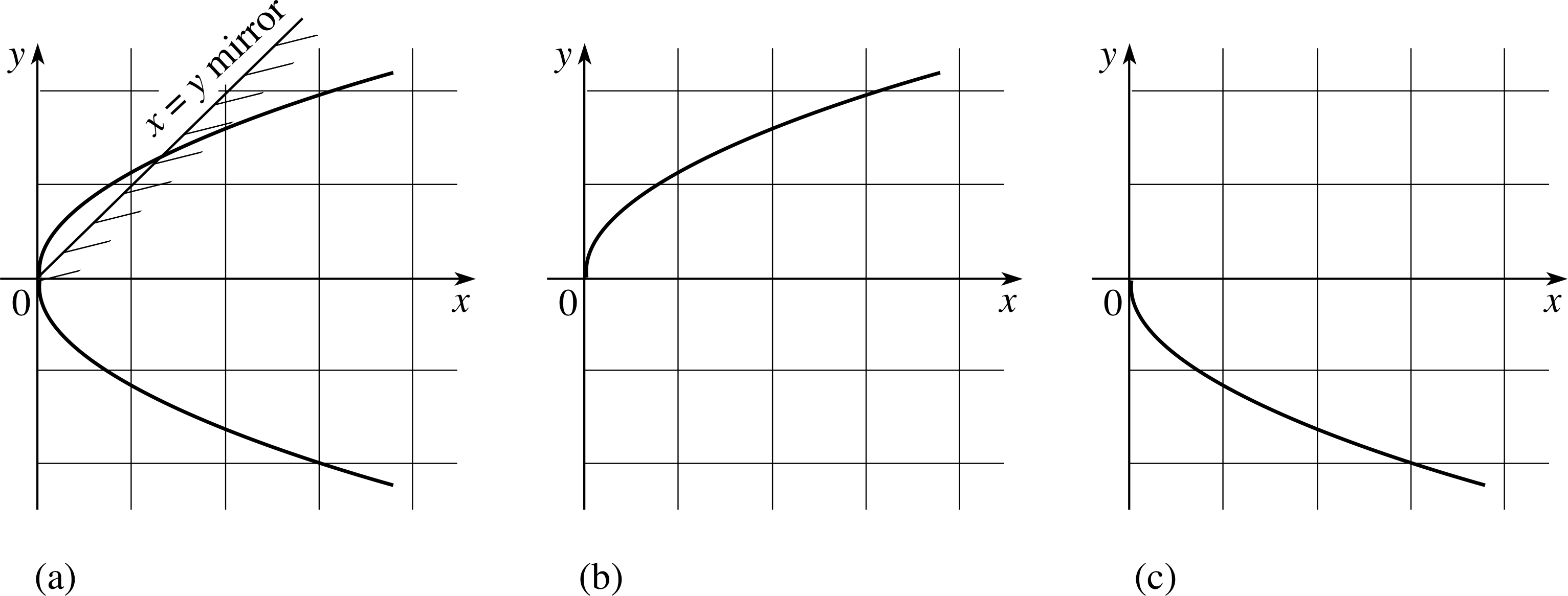
Figure 14 (a) The curve $y = \sqrt{x\os}$. (b) The curve $y = \left\lvert\,\sqrt{x\os}\,\right\rvert$ for x ≥ 0. (c) The curve $y = -\left\lvert\,\sqrt{x\os}\,\right\rvert$ for x ≥ 0.
Now you might be tempted to say that this is the graph of the function
$f(x) = \sqrt{x\os}$(27)
and that it is the inverse of g (x) since it ‘undoes’ the effect of g (x). However, a little more thought soon shows that the latter part of this claim cannot be true; f (x) does not really ‘undo’ the effect of g (x). If x = −2 then g (−2) = (−2)2 = 4 but $f(4) = \sqrt{4\os}$ = 2 or −2 so we are not unambiguously led back to the initial value of x. Moreover, the graph itself (Figure 14a) makes it clear that there are two values of y for each positive value of x and no values of y at all corresponding to negative values of x. The fact that two different value of y correspond to a single value of x means that Equation 27 does not actually define a function at all (since a function relates each value of the independent variable to a single value of the dependent variable). In fact, the function g (x) = x2 does not have an inverse. We have not shown this, but we have certainly demonstrated that $f(x) = \sqrt{x\os}$ is not the inverse.
Although $f(x) = \sqrt{x\os}$ is not really a function at all, such expressions are, mainly for historical reasons, often called multi–valued functions. This term is used to contrast them with true functions which can be described as single–valued functions. Of course, according to the definition given in Subsection 2.1, all functions are single-valued, so the term ‘single-valued function’, is actually a tautology and ‘multi-valued function’ is a misnomer.
Although $f(x) = \sqrt{x\os}$ is not a function it is fairly easy to find related expressions that can be used to define functions. For example
f+(x) = x for all x ≥ 0 i
andf−(x) = −x for all x ≥ 0
are both well defined (single–valued) functions. Their graphs are shown in Figures 14b and 14c, respectively. Furthermore, you should be able to convince yourself that f+(x) is the inverse of
g+(x) = x2 where x ≥ 0
while f− (x) is the inverse of the function
g−(x) = x2 where x ≤ 0
The need to restrict the domain of the function in this way is a common feature of the definition of many inverse functions. The general conclusion to be drawn from the above discussion is this:
In order for a function F (x) to have an inverse, a necessary condition that must be satisfied is that each value of F (x) must correspond to a unique value of x.
Figure 9 The cubic function g (x) = x3 − 4x.
Figure 8 The cubic function f (x) = x3.
Question T15
Look at Figures 8 and 9, illustrating the cubic functions defined by Equations 20 and 21, respectively. Do these functions have inverses? If so, how might they be defined?
Answer T15
The graph of Figure 8 shows that each value of y corresponds to a unique value of x. Thus there is no difficulty about defining the inverse function of Equation 20,
f (x) = x2(Eqn 20)
In fact it’s just $G(x) = \sqrt[{\large\raise{2pt}3}]{x\os}$.
Figure 9 shows a different situation. Each value of y does not correspond to a unique value of x, so it is not possible to define an inverse function.
Question T16
Would you expect a general quadratic function of the form f (x) = ax2 + bx + c to have an inverse? Explain your answer.
Answer T16
No. A particular value of f (x) may correspond to more than one value of x, so it is not possible to find an inverse function.
4.2 Functions of functions
It is often convenient to combine functions together; that is to start with an independent variable x, find the value of some function y = f (x) and then use that value of y as the argument of some other function z = g (y). This two–step process allows us to relate a single value of the dependent variable z to each value of the independent variable x, so z is related to x by a function. We can indicate this by writing z = h (x) where
h (x) = g (f (x))
The function h (x) is said to be a function of a function or a composite function. The idea is more common and more straightforward than it sounds; for example,
iff (x) = x2 and g (y) = 1/y where y ≠ 0
thenh (x) = g (f (x)) = g (x2) = 1/x2 where x ≠ 0
Note that in the final step we have simply taken the reciprocal of the argument of g (x2) – this is what the function g (y) = 1/y tells us to do – it doesn’t matter that the argument has been called x2 rather than y, simply take its reciprocal!
Question T17
Find g (f (x)) and f (g (x)) if f (x) = x + 2 and g (x) = 1/x. What is the largest possible domain for such a function, given that x is real?
Answer T17
g (f (x)) = g (x + 2) = 1/(x + 2) where x is any real number except −2.
f (g (x)) = f (1/x) = (1/x) + 2 where x ≠ 0.
Be careful to carry out the operations step by step and in the right order.
Question T18
Find g (h (f (y))) for the same f (x) and g (x) as in Question T17, and h (x) = x2.
Answer T18
g (h (f (y))) = g (h (y + 2)) = g ((y + 2)2) = 1/(y + 2)2 where y ≠ −2
Question T19
Suppose G (x) is the inverse of F (x), write down an explicit expression for the composite function H (x) = G (F (x)). (You do not need to know the explicit form of either function to answer this question.)
Answer T19
G (F (x)) = x since G (x) ‘undoes’ the effect of F (x) for every value of x in the domain of F (x). More formally, if we let y = F (x) and x = G (y),
H (x) = G (F (x)) = G (y) = x
5 Closing items
5.1 Module summary
- 1
-
A Section 2function consists of two sets and a rule, related in such a way that every element of the first set (the domain) is associated with a single element of the second set (the codomain).
- 2
-
The rule involved in a particular function is often presented in the form of an equation that may involve a number of Subsection 2.2variables, Subsection 2.2constants and Subsection 2.2parameters.
- 3
-
The sets involved in a particular function are often the sets of values of specific variables which may be continuous or discrete. Under these circumstances the values belonging to the first set (the domain) are said to be values of the Subsection 2.3independent variable(s) while the associated values belonging to the second set (the codomain) are said to be values of the Subsection 2.3dependent variable. This sort of functional relationship may be indicated by the equation y = f (x).
- 4
-
A Subsection 2.4table of values may be used to define a function of a discrete variable or to provide insight into the behaviour of a function of a continuous variable.
- 5
-
A Section 3graph, in which corresponding values of the independent and dependent variables are plotted as points on a pair of mutually perpendicular coordinate axes, provides a useful way of representing functions and equations. There are many standard conventions that apply to the drawing of graphs.
- 6
-
Subsection 3.4Linear functions of the form y = mx + c, where m is the Subsection 3.4gradient and c the Subsection 3.4intercept, have graphs that are Subsection 3.4straight lines. Graphically, m (= rise/run) determines the gradient of the line and c determines the point at which it intersects the y–axis. A straight line can be represented using a number of other forms, i.e. the gradient–intercept, point–gradient, two-point and intercept forms.
- 7
-
Subsection 3.5Quadratic functions of the form f (x) = a x2 + bx + c, have parabolic graphs that each have a single turning point known as the vertex of the parabola. The constants a, b and c determine the location of the vertex, $\dfrac{-b}{2a},\,\dfrac{-b^2}{4a}+c$, and the precise shape of the graph, including any values of x at which the curve meets or crosses (intersects) the x–axis, $x = \dfrac{-b\pm\sqrt{b^2-4ac}}{2a}$.
- 8
-
Subsection 3.6Polynomial functions of Subsection 3.6degree n have the form
f (x) = a0 + a1x + a2x2 + ... + an−2x n−2 + an−1x n−1 + anx n (with an ≠ 0)
Their graphs generally exhibit (local) maxima and (local) minima separated by points of inflection.
- 9
-
The Subsection 3.7reciprocal function, y = 1/x, has a graph that is a hyperbola and which exhibits asymptotes – lines that are approached by the graph as x or y approach large positive or negative values.
- 10
-
Given a function F (x), its Subsection 4.1inverse function G (x) ‘undoes’ the effect of F (x). So, if F (x) = y then G (y) = x for every value of x in the domain of F (x). For such a function to exist, each value of F (x) must correspond to a different (unique) value of x.
- 11
-
A Subsection 4.2function of a function or a composite function is a function of the form h (x) = g (f (x)).
5.2 Achievements
Having completed this module, you should be able to:
- A1
-
Define the terms that are emboldened and flagged in the margins of the module.
- A2
-
Describe the essential features of a function.
- A3
-
Explain the roles of constants, parameters and variables in a function.
- A4
-
Use equations to define functions and identify the independent and dependent variables in such definitions.
- A5
-
Set up a Cartesian coordinate system and use it to represent the properties of a function.
- A6
-
Plot an accurate graph of a given function.
- A7
-
Draw the graph of a linear function given the gradient and intercept, and find the gradient and intercept of a given graph.
- A8
-
Draw the graph of a linear function given either one point on the line and the gradient, or two points.
- A9
-
Sketch the graph of a quadratic function, rewrite the function in completed square form and hence identify the coordinates of its vertex, determine the number and location of any points at which the graph intersects the axes.
- A10
-
Sketch the graph of a cubic polynomial function, identify its point of inflection and any local maximum, or local minimum that it may have.
- A11
-
Draw the graph of the reciprocal function, and identify asymptotes in simple cases.
- A12
-
Recognize inverse functions (in simple cases), and distinguish between functions that may or may not have inverse functions.
- A13
-
Describe and identify the domain and codomain of a function.
- A14
-
Combine functions to produce a function of a function (in simple cases).
Study comment You may now wish to take the Exit test for this module which tests these Achievements. If you prefer to study the module further before taking this test then return to the Module contents to review some of the topics.
5.3 Exit test
Study comment Having completed this module, you should be able to answer the following questions each of which tests one or more of the Achievements.
Question E1 (A4 and A5)
A function f (x) is defined by
f (x) = x for x ≥ 0, and f (x) = −x for x < 0.
Plot a graph of f (x) for values of x between −4 and +4.
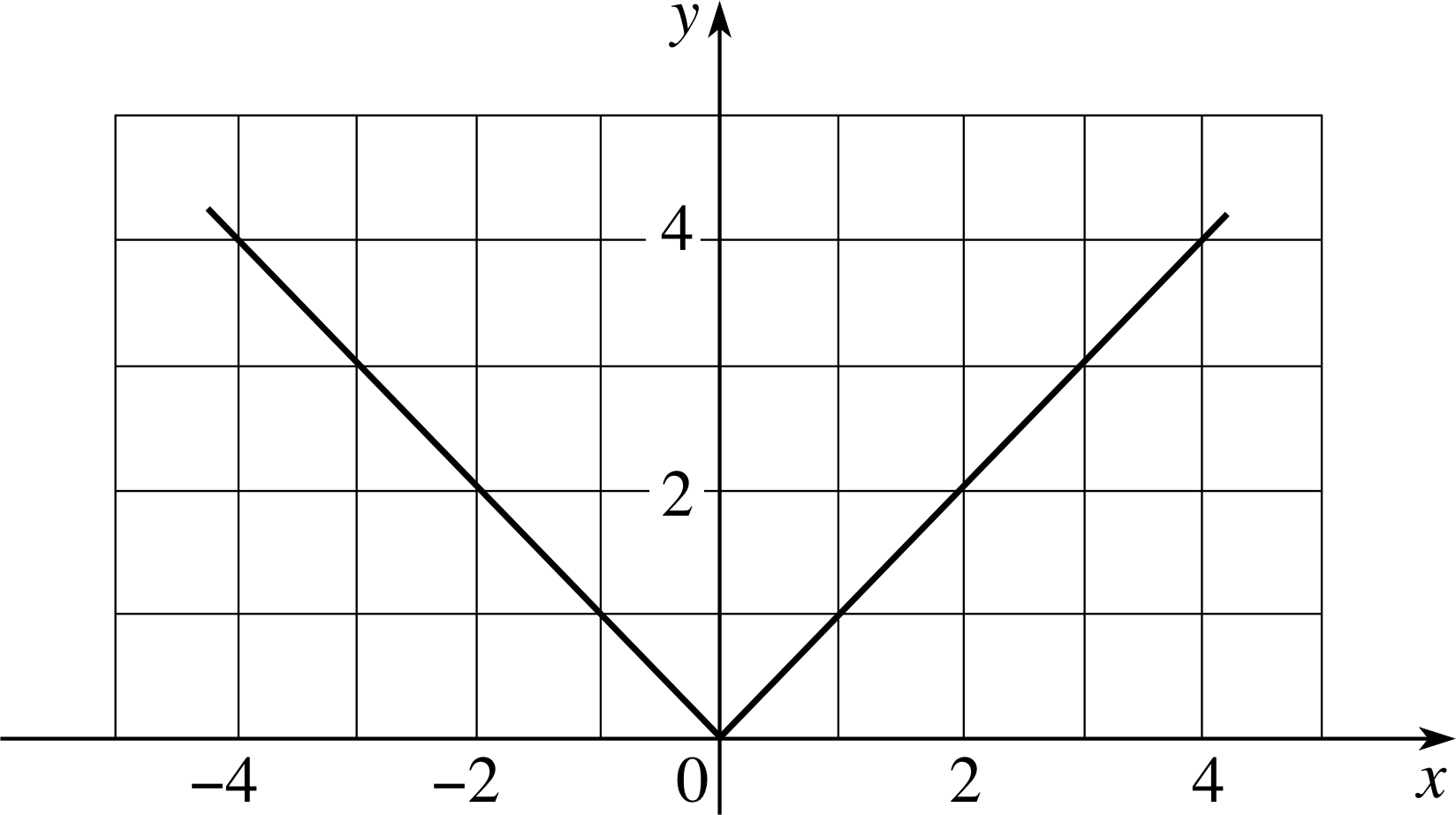
Figure 20 See Answer E1.
Answer E1
The graph of the function f (x) is given in Figure 20.
In this case there is a definite kink at the origin. The function can be defined as f (x) = | x |.
(Reread Subsection 2.4Subsections 2.4, Subsection 3.13.1 and Subsection 3.23.2 if you had difficulty with this question.)
Question E2 (A5 and A7)
Sketch graphs of the following functions:
f (x) = 2x, f (x) = 2x + 3, f (x) = 2x − 1, f (x) = −½x
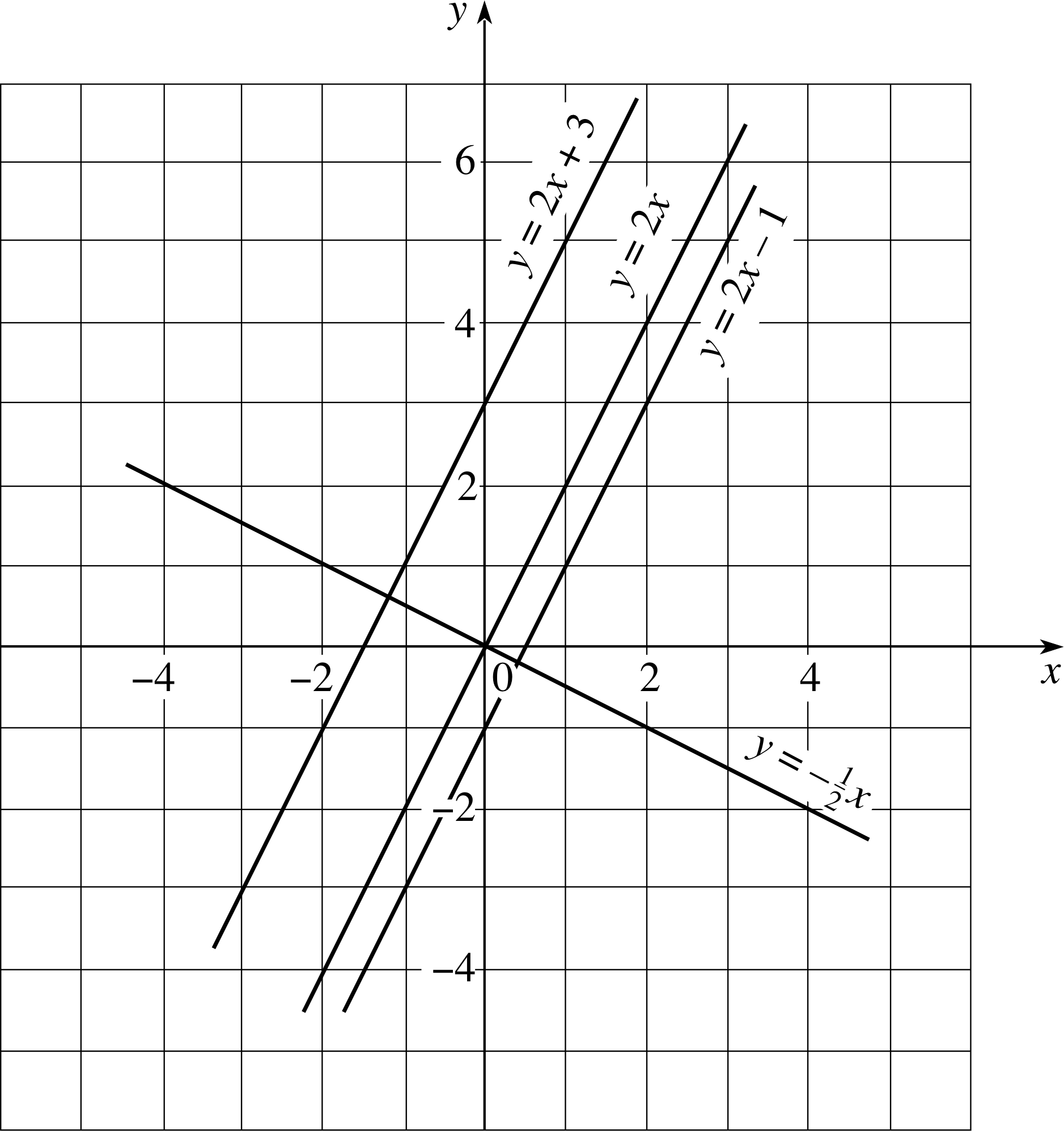
Figure 21 See Answer E2.
Answer E2
See the sketches in Figure 21
(Reread Subsection 3.1Subsections 3.1, Subsection 3.23.2, Subsection 3.33.3 and Subsection 3.43.4 if you had difficulty with this question.)
Question E3 (A8)
What is the equation of the straight line (in the form y = mx + c) which passes through the point (3, 5) with gradient 3?
Answer E3
Using the point–gradient form of the equation of a straight line,
(y − 5)/(x − 3) = 3; so y − 5 = 3 (x − 3), i.e. y = 3x − 4
(Reread Subsection 3.4 if you had difficulty with this question.)
Question E4 (A8)
Give the equation (in gradient–intercept form) of the straight line which passes through the points (−1, 5) and (2, −1).
Answer E4
Using the two–point form of the equation of a straight line,
(y − 5)/(x + 1) = (−1 − 5)/(2 + 1) = −16/3 = −2
soy = −2x + 3
(Reread Subsection 3.4 if you had difficulty with this question.)
Question E5 (A9)
Three quadratic functions are defined by the following:
f (x) = ½x2 − 3, g (x) = −½x2 + 1, h (x) = x2 + 2x + 2
What are the coordinates of their vertices? Which of the curves intersect the x–axis and where do such intersections occur? Sketch the graphs of the three functions on a single pair of axes.
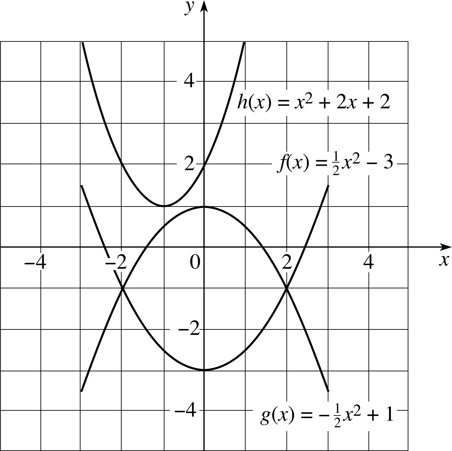
Figure 22 See Answer E5.
Answer E5
y f (x) is in completed square form (Equation 14) and has its vertex at (0, −3); g (x) is also in completed square form and its vertex is at (0, 1); h (x) may be written in completed square form as h (x) = (x + 1)2 + 1 and has its vertex at (−1, 1).
f (x) and g (x) both intersect the x–axis twice since they both have discriminants that are greater than zero. h (x) has a negative discriminant, so it does not cut the axis. For f (x) the points of intersection are x = ±6, and for g (x) they are x = ±2. (These values may be obtained from Equation 17, but in this case it is easier to deduce them directly from the given functions.)
$x = \dfrac{-b\pm\sqrt{b^2-4ac}}{2a}$(Eqn 17)
The graphs are shown in Figure 22.
(Reread Subsection 3.5 if you had difficulty with this question.)
Question E6 (A10)
Sketch the graphs of y = (x − 1)3 and y = x3 − 9x.
In each case, how many times does the curve cross the x–axis? Where are the points of inflection located?
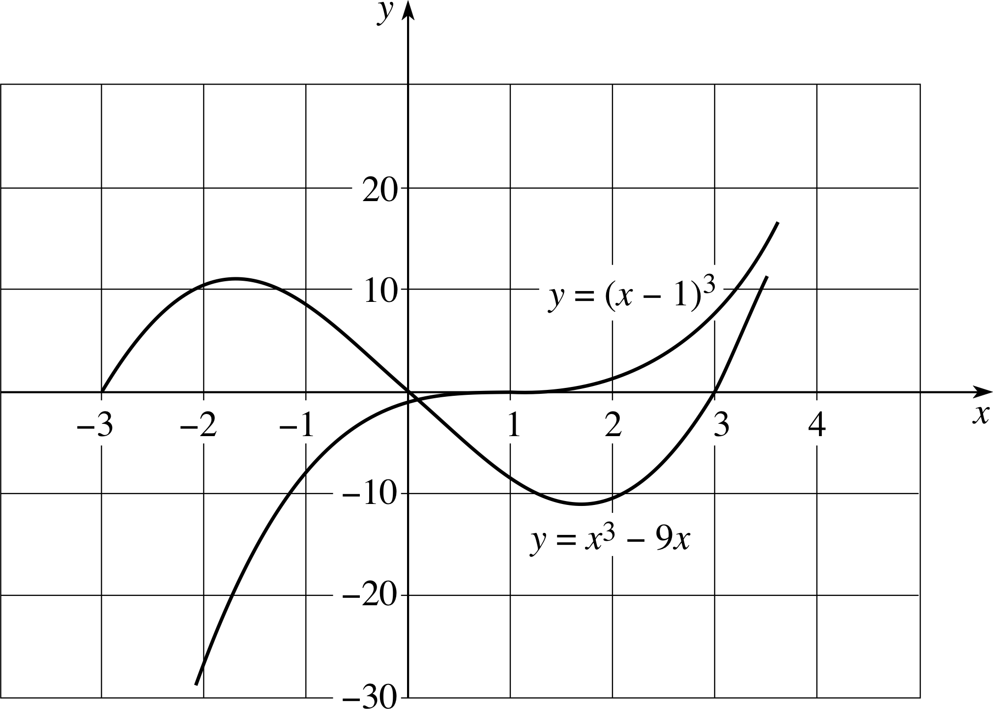
Figure 23 See Answer E6.
Answer E6
The sketch of y = (x − 1)3 is given in Figure 23. The curve y = (x− 1)3 is the same shape as the curve in Figure 8, but it has been displaced along the x–axis by 1 scale unit to the right. (If we had let (x − 1) = X we would have been plotting y = X3). The curve crosses the x–axis once. Its point of inflection is at (1, 0).
The curve y = x3 − 9x is similar to that of Figure 9; it crosses the x–axis three times and has a point of inflection at the origin. (The fact that the point of inflection is close to the origin in this case should be obvious from your graph. However, the proof that this is its exact location is beyond the scope of this module.)
(Reread Subsection 3.6 if you had difficulty with this question.)
Question E7 (A5, A6 and A7)
The vertical velocity of a stone, thrown vertically upwards from the ground, is given by
υ = u0 − gt
where u0 is the initial velocity of the stone and g is a constant. Assuming g = 10 m s−2 upwards and u0 = 20 m s−1, draw a properly labelled graph showing υ as a function of t for the first 4 seconds of flight.
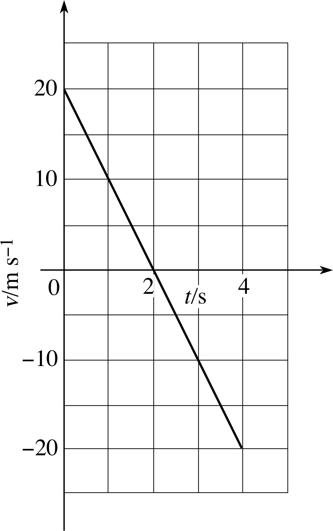
Figure 24 See Answer E7.
Answer E7
See Figure 24. (Note the inclusion of SI units in the axis labels.) After the first two seconds the velocity becomes negative, i.e. the stone is moving downwards.
(Reread Subsection 3.3 and Subsection 3.43.4 if you had difficulty with this question.)
Question E8 (A5 and A9)
At time t, the stone mentioned in Question E7 is at a height h above the ground where
h = ut − ½gt2
Draw a graph of h as a function of t and find (a) the maximum height the stone reaches, and (b) the time before it hits the ground. What features of the graph determined your answers?
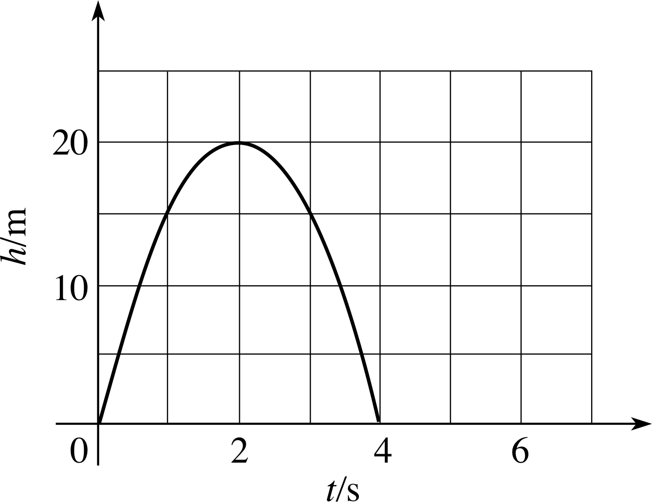
Figure 25 See Answer E8.
Answer E8
The graph of the function is given in Figure 25.
(a) The maximum height (determined by the vertex of the parabola) is 20 m.
(b) The total time (determined by the difference in the t values at the two points of intersection with the t–axis) is 4 s.
(Reread Subsection 3.5 if you had difficulty with this question.)
Question E9 (A11 and A12)
Sketch the graph of the function $f(x) = \left\lvert\,\sqrt{x^2+1}\,\right\rvert$
Does this curve have asymptotes? Does f (x) have an inverse function?
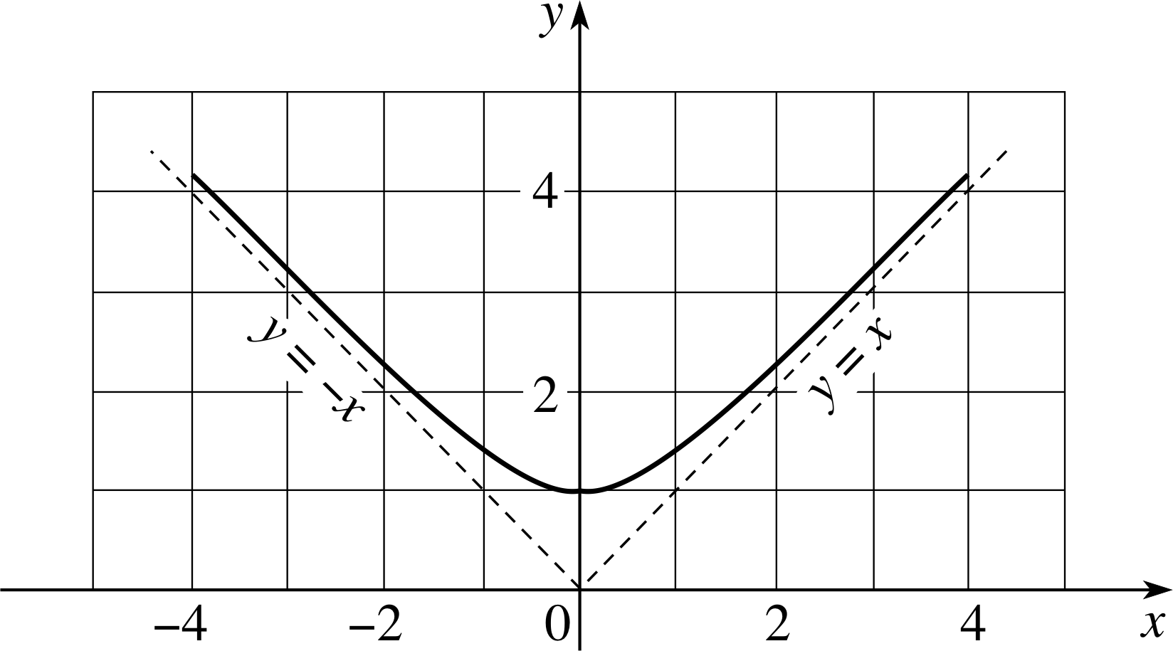
Figure 26 See Answer E9.
Answer E9
The graph of the function is given in Figure 26. As x becomes larger and larger (either positively or negatively), the expression under the square root symbol gets closer and closer to x2, so, f (x) ≈ | x | for large values of x. You determined the shape of this function in Question E1, thus the asymptotes are the lines y = x and y = −x, and the curve approaches each of them from above. The function f (x) does not have an inverse because a particular value of f (x) may correspond to several different values of x.
(Reread Subsection 3.7Subsections 3.7 and Subsection 4.14.1 if you had difficulty with this question.)
Question E10 (A13 and A14)
If f (x) = (x − 1)2 and g (x) = x + 1, what are f (g (y)) and g (f (y))?
If y is real, what are the largest possible domains for these functions?
Answer E10
f (g (y)) = f (y + 1) = y2, where y may be any real number g (f (y)) = g ((y − 1)2) = (y−1)2 + 1 = y2 − 2y + 2, where y may be any real number.
(Reread Subsection 4.2Subsections 4.2 and Subsection 2.32.3 if you had difficulty with this question.)
Study comment This is the final Exit test question. When you have completed the Exit test go back and try the Subsection 1.2Fast track questions if you have not already done so.
If you have completed both the Fast track questions and the Exit test, then you have finished the module and may leave it here.
Study comment Having seen the Fast track questions you may feel that it would be wiser to follow the normal route through the module and to proceed directly to the following Ready to study? Subsection.
Alternatively, you may still be sufficiently comfortable with the material covered by the module to proceed directly to the Section 5Closing items.